This video is pretty good, and I thought that I’d add some equations to the explanation:
So, in terms of the mathematics, what is going on?
The graph they came up with is “new confirmed cases” on the y-axis (log scale) and total number of cases on the x-axis. Let’s see what this looks like for exponential growth.
Here, letting the total number of cases at time be denoted by , the number of new cases is , the first derivative.
In the case of exponential growth, where is positive.
which is what is being plotted on the y-axis. So with the change of variable we are letting and our new function is , which, of course, is a straight line through the origin. That is, of course, IF the growth is exponential.
To get a feel for what this looks like, suppose we had polynomial growth; say . Then In the case of linear growth we’d have (constant) and for, say, , or a “concave down” function.
Now for the logistic situation in which the number of cases grows exponentially at first and then starts to level out to some steady state value, call it , the relationship between the number of cases and the new number of cases looks like so our which is a quadratic which opens down.
Let’s start with an example from sports: basketball free throws. At a certain times in a game, a player is awarded a free throw, where the player stands 15 feet away from the basket and is allowed to shoot to make a basket, which is worth 1 point. In the NBA, a player will take 2 or 3 shots; the rules are slightly different for college basketball.
Each player will have a “free throw percentage” which is the number of made shots divided by the number of attempts. For NBA players, the league average is .672 with a variance of .0074.
Now suppose you want to determine how well a player will do, given, say, a sample of the player’s data? Under classical (aka “frequentist” ) statistics, one looks at how well the player has done, calculates the percentage () and then determines a confidence interval for said : using the normal approximation to the binomial distribution, this works out to
\
Yes, I know..for someone who has played a long time, one has career statistics ..so imagine one is trying to extrapolate for a new player with limited data.
That seems straightforward enough. But what if one samples the player’s shooting during an unusually good or unusually bad streak? Example: former NBA star Larry Bird once made 71 straight free throws…if that were the sample, with variance zero! Needless to say that trend is highly unlikely to continue.
Classical frequentist statistics doesn’t offer a way out but Bayesian Statistics does.
This is a good introduction:
But here is a simple, “rough and ready” introduction. Bayesian statistics uses not only the observed sample, but a proposed distribution for the parameter of interest (in this case, p, the probability of making a free throw). The proposed distribution is called a prior distribution or just prior. That is often labeled
Since we are dealing with what amounts to 71 Bernoulli trials where p = .672 so the distribution of each random variable describing the outcome of each individual shot has probability mass fuction where for a make and for a miss.
Our goal is to calculate what is known as a posterior distribution (or just posterior) which describes after updating with the data; we’ll call that .
How we go about it: use the principles of joint distributions, likelihood functions and marginal distributions to calculate
The denominator “integrates out” p to turn that into a marginal; remember that the are set to the observed values. In our case, all are 1 with .
What works well is to use the beta distribution for the prior. Note: the pdf is and if one uses , this works very well. Now because the mean will be and given the required mean and variance, one can work out algebraically.
Now look at the numerator which consists of the product of a likelihood function and a density function: up to constant , if we set we get
The denominator: same thing, but gets integrated out and the constant cancels; basically the denominator is what makes the fraction into a density function.
So, in effect, we have which is just a beta distribution with new .
So, I will spare you the calculation except to say that that the NBA prior with leads to
Yes, shifted to the right..very narrow as well. The information has changed..but we avoid the absurd contention that with a confidence interval of zero width.
We can now calculate a “credible interval” of, say, 90 percent, to see where most likely lies: use the cumulative density function to find this out:
And note that . In fact, Bird’s lifetime free throw shooting percentage is .882, which is well within this 91.6 percent credible interval, based on sampling from this one freakish streak.
Some time ago, I served in the U. S. Navy. The world “Navy” was said to be an acronym for Never Again Volunteer Yourself. But I forgot that and volunteered to teach a class on Mathematical interest theory. That means, of course, I have to learn some of this, and so I am going over a classic text and doing the homework.
The math itself is pretty simple, but some of the concepts seem strange to me at this time. So, I’ll be using this as “self study” prior to the start of the semester, and perhaps I’ll put more notes up as I go along.
By the way, if you are interested in the notes for my undergraduate topology class, you can find them here.
Discounting: concepts, etc. (from this text) (Kellison)
Initial concept:
Suppose you borrow 100 dollars for one year at 8 percent interest. So at time 0 you have 100 dollars and at time 1, you pay back 100 + (100)(.08) = 108.
Now let’s do something similar via “discounting”. The contract is for 100 dollars and the rate is an 8 percent discount. The bank takes their 8 percent AT THE START and you end up with 92 dollars at time zero and pay back 100 at time 1.
So the difference is: in interest, the interest is paid upon pay back, and so the amount function is: . In the discount situation we have where is the discount rate. So the amount function is where
If we used compound interest, we’d have and in compound discount we’d have
This leads to some interesting concepts.
First of all, there is the “equivalence concept”. Think about the above example: if getting 92 dollars now lead to 100 dollars after one period, what interest rate would that be? Of course it would be . So what we’d have is this: or .
Effective rates: this is only of interest in the “simple interest” or “simple discount” situation.
Let’s start with simple interest. The amount function is of the form . The idea is that if you invest, say, 100 dollars earning, say, 5 percent simple interest (NO compounding), then in one year you get 5 dollars of interest, 2 years, 10 dollars of interest, 3 years 15 dollars of interest, etc. You can see the problem here; say at the end of year one your account was worth 105 dollars and at the end of year 2, it was worth 110 dollars. So, in effect, your 105 dollars earned 5 dollars interest in the second year. Effectively, you earned a lower rate in year 2. It got worse in year 3 (110 earned only 5 dollars).
So the EFFECTIVE INTEREST in period is which you can see goes to zero as goes to infinity.
Effective discount works in a similar manner, though we divide by the amount at the end of the period, rather than the beginning of it:
I admit that I chuckled when a famous stand up comic said: “”New Rule: Any teacher that says, ‘I learn as much from my students as they learn from me,’ is a sh***y teacher and must be fired.””
Yes, I assure you, when it comes to subject matter, my students had bloody well learn more from me than I do from them. 🙂
BUT: when it comes to class preparation, I find myself learning a surprising amount of material, even when I’ve taught the class before.
For example, teaching third semester calculus (multi-variable) lead me to thinking about some issues and to my rediscovering some theorems presented a long time ago and often not used in calculus/advanced calculus books. THAT lead to a couple of published papers.
And, given that my teaching specialty has morphed into applied mathematics, teaching numerical analysis has lead me to learn some interesting stuff for the first time; it has filled some of the “set of measure infinity” gaps in my mathematical education.
So, ok, this semester I am teaching elementary topology. Surely, I’d learn nothing new though I’d enjoy myself. It turns out: that isn’t the case. Very often I find myself starting to give a proof of something and find myself making (correct) assumptions that, well, I last proved 30 years ago. Then I ask myself: “now, just why is this true again?”
One of the fun projects is showing that the topologist’s sine curve is connected but not path connected (if one adds the vertical segment at x = 0). It turns out that this proof is pretty easy, BUT…I found myself asking “why is this detail true?” a ton of times. I drove myself crazy.
Note: later today I’ll give my favorite proof; it uses the sequential definition of continuity and the subspace topology; both of these concepts are new to my students and so it is helpful to find reasons to use them, even if these aren’t the most mathematically elegant ways to do the proof.
This is why I proved the Intermediate Value Theorem using the “least upper bound” concept instead of using connectivity. The more they use a new concept, the better they understand it.
I follow Schneier’s Security Blog. Today, he alerted his readers to this post about an NSA member’s take on the cryptography session of a mathematics conference. The whole post is worth reading, but these comments really drive home some of the tension between those of us in academia :
Alfredo DeSantis … spoke on “Graph decompositions and secret-sharing schemes,” a silly topic which brings joy to combinatorists and yawns to everyone else. […]
Perhaps it is beneficial to be attacked, for you can easily augment your publication list by offering a modification.
[…]
This result has no cryptanalytic application, but it serves to answer a question which someone with nothing else to think about might have asked.
[…]
I think I have hammered home my point often enough that I shall regard it as proved (by emphatic enunciation): the tendency at IACR meetings is for academic scientists (mathematicians, computer scientists, engineers, and philosophers masquerading as theoretical computer scientists) to present commendable research papers (in their own areas) which might affect cryptology at some future time or (more likely) in some other world. Naturally this is not anathema to us.
I freely admit this: when I do research, I attack problems that…interests me. I don’t worry if someone else finds them interesting or not; when I solve such a problem I submit it and see if someone else finds it interesting. If I solved the problem correctly and someone else finds it interesting: it gets published. If my solution is wrong, I attempt to fix the error. If no one else finds it interesting, I work on something else. 🙂
I had Dfield8 from MATLAB propose solutions to meeting the following initial conditions:
.
Now, of course, one of these solutions is non-unique. But, of all of the solutions drawn: do you trust ANY of them? Why or why not?
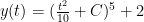
Note: you really don’t have to do much calculus to see what is wrong with at least one of these. But, if you must know, the general solution is given by (and, of course, the equilibrium solution ). But that really doesn’t provide more information that the differential equation does.
By the way, here are some “correct” plots of the solutions, (up to uniqueness)
Chebyshev (or Tchebycheff) polynomials are a class of mutually orthogonal polynomials (with respect to the inner product: ) defined on the interval . Yes, I realize that this is an improper integral, but it does converge in our setting.
These are used in approximation theory; here are a couple of uses:
1. The roots of the Chebyshev polynomial can be used to find the values of that minimize the maximum of over the interval . This is important in minimizing the error of the Lagrange interpolation polynomial.
2. The Chebyshev polynomial can be used to adjust an approximating Taylor polynomial to increase its accuracy (away from the center of expansion) without increasing its degree.
Let’s discuss the polynomials themselves. They are defined for all positive integers as follows:
. Now, it is an interesting exercise in trig identities to discover that these ARE polynomials to begin with; one shows this to be true for, say, by using angle addition formulas and the standard calculus resolution of things like . Then one discovers a relation: to calculate the rest.
The definition allows for some properties to be calculated with ease: the zeros occur when and the first derivative has zeros where ; these ALL correspond to either an endpoint max/min at or local max and mins whose values are also . Here are the graphs of
Now here is a key observation: the graph of a forms spanning arcs in the square and separates the square into regions. So, if there is some other function whose graph is a connected, piecewise smooth arc that is transverse to the graph of that both spans the square from to and that stays within the square, that graph must have points of intersection with the graph of .
Now suppose that is the graph of a polynomial of degree whose leading coefficient is and whose graph stays completely in the square . Then the polynomial has degree (because the leading terms cancel via the subtraction) but has roots (the places where the graphs cross). That is clearly impossible; hence the only such polynomial is .
This result is usually stated in the following way: is normalized to be monic (have leading coefficient 1) by dividing the polynomial by and then it is pointed out that the normalized is the unique monic polynomial over that stays within for all . All other monic polynomials have a graph that leaves that box at some point over .
Of course, one can easily cook up analytic functions which don’t leave the box but these are not monic polynomials of degree .
For us, calculus III is the most rushed of the courses, especially if we start with polar coordinates. Getting to the “three integral theorems” is a real chore. (ok, Green’s, Divergence and Stoke’s theorem is really just but that is the subject of another post)
But watching this lecture made me wonder: should I say a few words about how to calculate a convolution integral?
In the context of Fourier Transforms, the convolution integral is defined as it was in analysis class: . Typically, we insist that the functions be, say, and note that it is a bit of a chore to show that the convolution of two functions is ; one proves this via the Fubini-Tonelli Theorem.
(The straight out product of two functions need not be ; e.g, consider for and zero elsewhere)
So, assuming that the integral exists, how do we calculate it? Easy, you say? Well, it can be, after practice.
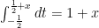
But to test out your skills, let be the function that is for and zero elsewhere. So, what is ???
So, it is easy to see that only assumes the value of on a specific region of the plane and is zero elsewhere; this is just like doing an iterated integral of a two variable function; at least the first step. This is why it fits well into calculus III.
for the following region:
This region is the parallelogram with vertices at .
Now we see that we can’t do the integral in one step. So, the function we are integrating has the following description:
So the convolution integral is for and for .
That is, of course, the tent map that we described here. The graph is shown here:
So, it would appear to me that a good time to do a convolution exercise is right when we study iterated integrals; just tell the students that this is a case where one “stops before doing the outside integral”.
The context: one is showing that the Fourier transform of the convolution of two functions is the product of the Fourier transforms (very similar to what happens in the Laplace transform); that is where
So, during this lecture, Osgood shows that ; that is, this modified Gaussian function is “its own Fourier transform”.
I’ll sketch out what he did in the lecture at the end of this post. But just for fun (and to make a point) I’ll give a method that uses an elementary residue integral.
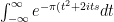
Both methods start by using the definition:
Method 1: combine the exponential functions in the integrand:
. Now complete the square to get:
Now factor out the factor involving alone and write as a square:
Now, make the substitution to obtain:
Now we show that the above integral is really equal to
To show this, we perform along the retangular path : and let
Now the integral around the contour is 0 because is analytic.
We wish to calculate the negative of the integral along the top boundary of the contour. Integrating along the bottom gives 1.
As far as the sides: if we fix we note that and the magnitude goes to zero as So the integral along the vertical paths approaches zero, therefore the integrals along the top and bottom contours agree in the limit and the result follows.
Method 2: The method in the video
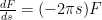
This uses “differentiation under the integral sign”, which we talk about here.
Stat with and note
Now we do integration by parts: and the integral becomes:
Now the first term is zero for all values of as . The second term is merely:
.
So we have shown that which is a differential equation in which has solution (a simple separation of variables calculation will verify this). Now to solve for the constant note that .
The result follows.
Now: which method was easier? The second required differential equations and differentiating under the integral sign; the first required an easy residue integral.
By the way: the video comes from an engineering class. Engineers need to know this stuff!


 ) and then determines a confidence interval for said
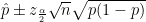
 with variance zero! Needless to say that trend is highly unlikely to continue.
 where
where  for a make and
  for a miss.
  after updating with the data; we’ll call that
  .
.
 are set to the observed values. In our case, all are 1 with
  .
.  and if one uses
  , this works very well. Now because the mean will be
  and
and  given the required mean and variance, one can work out
  algebraically.
  we get
 which is just a beta distribution with new
  .
. leads to
 .
.

 with a confidence interval of zero width.
 . In fact, Bird’s lifetime free throw shooting percentage is .882, which is well within this 91.6 percent credible interval, based on sampling from this one freakish streak.
  . In the discount situation we have
  where
where  is the discount rate. So the amount function is
  where
where 
 and in compound discount we’d have
 . So what we’d have is this:
  or
or  .
. . The idea is that if you invest, say, 100 dollars earning, say, 5 percent simple interest (NO compounding), then in one year you get 5 dollars of interest, 2 years, 10 dollars of interest, 3 years 15 dollars of interest, etc. You can see the problem here; say at the end of year one your account was worth 105 dollars and at the end of year 2, it was worth 110 dollars. So, in effect, your 105 dollars earned 5 dollars interest in the second year. Effectively, you earned a lower rate in year 2. It got worse in year 3 (110 earned only 5 dollars).
 is
is  which you can see goes to zero as
 meeting the following initial conditions:
 .
.
 (and, of course, the equilibrium solution
  ). But that really doesn’t provide more information that the differential equation does.
 ) defined on the interval
 ![[-1, 1]](https://s0.wp.com/latex.php?latex=%5B-1%2C+1%5D+&bg=ffffff&fg=000000&s=0&c=20201002) . Yes, I realize that this is an improper integral, but it does converge in our setting.
. Yes, I realize that this is an improper integral, but it does converge in our setting.![x_0, x_1, x_2, ...x_k \in [-1,1]](https://s0.wp.com/latex.php?latex=x_0%2C+x_1%2C+x_2%2C+...x_k+%5Cin+%5B-1%2C1%5D+&bg=ffffff&fg=000000&s=0&c=20201002) that minimize the maximum of
that minimize the maximum of  over the interval
 ![[-1,1]](https://s0.wp.com/latex.php?latex=%5B-1%2C1%5D+&bg=ffffff&fg=000000&s=0&c=20201002) . This is important in minimizing the error of the
. This is important in minimizing the error of the  to increase its accuracy (away from the center of expansion) without increasing its degree.
 . Now, it is an interesting exercise in trig identities to discover that these ARE polynomials to begin with; one shows this to be true for, say,
  by using angle addition formulas and the standard calculus resolution of things like
  . Then one discovers a relation:
  to calculate the rest.
  definition allows for some properties to be calculated with ease: the zeros occur when
  and the first derivative has zeros where
  ; these ALL correspond to either an endpoint max/min at
  or local max and mins whose
  values are also
  . Here are the graphs of


 forms
forms ![[-1, 1] \times [-1,1]](https://s0.wp.com/latex.php?latex=%5B-1%2C+1%5D+%5Ctimes+%5B-1%2C1%5D+&bg=ffffff&fg=000000&s=0&c=20201002) and separates the square into
and separates the square into  regions. So, if there is some other function
  whose graph is a connected, piecewise smooth arc that is transverse to the graph of
  to
to  and that stays within the square, that graph must have
  is the graph of a polynomial of degree
  and whose graph stays completely in the square
  has degree
  (because the leading terms cancel via the subtraction) but has
  .
. is normalized to be monic (have leading coefficient 1) by dividing the polynomial by
 ![[-\frac{1}{2^{n-1}}, \frac{1}{2^{n-1}}]](https://s0.wp.com/latex.php?latex=%5B-%5Cfrac%7B1%7D%7B2%5E%7Bn-1%7D%7D%2C+%5Cfrac%7B1%7D%7B2%5E%7Bn-1%7D%7D%5D&bg=ffffff&fg=000000&s=0&c=20201002) for all
for all ![x \in [-1,1]](https://s0.wp.com/latex.php?latex=x+%5Cin+%5B-1%2C1%5D+&bg=ffffff&fg=000000&s=0&c=20201002) . All other monic polynomials have a graph that leaves that box at some point over
. All other monic polynomials have a graph that leaves that box at some point over  but that is the subject of another post)
 . Typically, we insist that the functions be, say,
  and note that it is a bit of a chore to show that the convolution of two
  for
for ![x \in (0,1]](https://s0.wp.com/latex.php?latex=x+%5Cin+%280%2C1%5D+&bg=ffffff&fg=000000&s=0&c=20201002) and zero elsewhere)
and zero elsewhere)  be the function that is
  for
for ![x \in [\frac{-1}{2}, \frac{1}{2}]](https://s0.wp.com/latex.php?latex=x+%5Cin+%5B%5Cfrac%7B-1%7D%7B2%7D%2C+%5Cfrac%7B1%7D%7B2%7D%5D+&bg=ffffff&fg=000000&s=0&c=20201002) and zero elsewhere. So, what is
and zero elsewhere. So, what is  ???
??? only assumes the value of
  plane and is zero elsewhere; this is just like doing an iterated integral of a two variable function; at least the first step. This is why it fits well into calculus III.
 for the following region:
 .
. 
 has the following description:
![f(x-t)f(t)=\left\{\begin{array}{c} 1,x \in [-1,0], -\frac{1}{2} t \le \frac{1}{2}+x \\ 1 ,x\in [0,1], -\frac{1}{2}+x \le t \le \frac{1}{2} \\ 0 \text{ elsewhere} \end{array}\right.](https://s0.wp.com/latex.php?latex=f%28x-t%29f%28t%29%3D%5Cleft%5C%7B%5Cbegin%7Barray%7D%7Bc%7D+1%2Cx+%5Cin+%5B-1%2C0%5D%2C+-%5Cfrac%7B1%7D%7B2%7D+t+%5Cle+%5Cfrac%7B1%7D%7B2%7D%2Bx+%5C%5C+1+%2Cx%5Cin+%5B0%2C1%5D%2C+-%5Cfrac%7B1%7D%7B2%7D%2Bx+%5Cle+t+%5Cle+%5Cfrac%7B1%7D%7B2%7D+%5C%5C+0+%5Ctext%7B+elsewhere%7D+%5Cend%7Barray%7D%5Cright.++&bg=ffffff&fg=000000&s=0&c=20201002)
 for
for  and
and  for
for ![x \in [0,1]](https://s0.wp.com/latex.php?latex=x+%5Cin+%5B0%2C1%5D+&bg=ffffff&fg=000000&s=0&c=20201002) .
.
 where
where 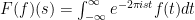 provided the integral converges.
  ; one can check that
  . One way is to use the fact that
  and do the substitution
  ; of course one should be able to
  ; that is, this modified Gaussian function is “its own Fourier transform”.
 . Now complete the square to get:
 alone and write as a square:
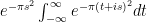
 to obtain:

 along the retangular path
  :
:  and let

 is analytic.
  and the magnitude goes to zero as
 and the integral becomes:
 . The second term is merely:
 .
. which is a differential equation in
  (a simple separation of variables calculation will verify this). Now to solve for the constant
  note that
 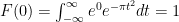 .
. 