College Math Teaching

March 26, 2023

Annoying calculations: Beta integral

March 7, 2023

Teaching double integrals: why you should *always* sketch the region

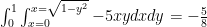
The problem (from Larson’s Calculus, an Applied Approach, 10’th edition, Section 7.8, no. 18 in my paperback edition, no. 17 in the e-book edition) does not seem that unusual at a very quick glance:

\int^2_0 \int^{\sqrt{1-y^2}}_0 -5xy dx dy if you have a hard time reading the image. AND, *if* you just blindly do the formal calculations:

-{5 \over 2} \int^2_0 x^2y|^{x=\sqrt{1-y^2}}_{x=0}  dy = -{5 \over 2} \int^2_0 y-y^3 dy = -{5 \over 2}(2-4) = 5 which is what the text has as “the answer.”

But come on. We took a function that was negative in the first quadrant, integrated it entirely in the first quadrant (in standard order) and ended up with a positive number??? I don’t think so!

Indeed, if we perform \int^2_0 \int^1_0 -5xy dxdy =-5 which is far more believable.

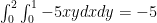
So, we KNOW something is wrong. Now let’s attempt to sketch the region first:

Oops! Note: if we just used the quarter circle boundary we obtain

\int^1_0 \int^{x=\sqrt{1-y^2}}_{x=0} -5xy dxdy = -{5 \over 8}

The 3-dimensional situation: we are limited by the graph of the function, the cylinder x^2+y^2 =1 and the planes y=0, x =0 ; the plane y=2 is outside of this cylinder. (from here: the red is the graph of z = -5xy

Now think about what the “formal calculation” really calculated and wonder if it was just a coincidence that we got the absolute value of the integral taken over the rectangle 0 \leq x \leq 1, 0 \leq y \leq 2

September 13, 2021

Integrals of functions with nice inverses

This idea started as a bit of a joke:

Of course, for readers of this blog: easy-peasy. u =\sqrt{tan(x)} \rightarrow u^2 =tan(x) \rightarrow x = arctan(u^2), dx = {2udu \over 1+u^4} so the integral is transformed into \int {2u^2 \over 1+u^4} du and so we’ve entered the realm of rational functions. Ok, ok, there is some work to do.

But for now, notice what is really doing on: we have a function under the radical that has an inverse function (IF we are careful about domains) and said inverse function has a derivative which is a rational function

More shortly: let f(x) be such that {d \over dx} f^{-1}(x) = q(x) then:

\int (f(x))^{1 \over n} dx gets transformed: u^n = f(x) \rightarrow x =f^{-1}(u^n) and then dx = nu^{n-1}q(u^n) and the integral becomes \int n u^n q(u^n) du which is a rational function integral.

Yes, yes, we need to mind domains.

July 14, 2020

An alternative to trig substitution, sort of..

Ok, just for fun: \int \sqrt{1+x^2} dx =

The usual is to use x =tan(t), dx =sec^2(t) dt which transforms this to the dreaded \int sec^3(t) dt integral, which is a double integration by parts.
Is there a way out? I think so, though the price one pays is a trickier conversion back to x.

Let’s try x =sinh(t) \rightarrow dx = cosh(t) dt so upon substituting we obtain \int |cosh(t)|cosh(t) dt and noting that cosh(t) > 0 alaways:

\int cosh^2(t)dt Now this can be integrated by parts: let u=cosh(t) dv = cosh(t) dt \rightarrow du =sinh(t), v = sinh(t)

So \int cosh^2(t)dt = cosh(t)sinh(t) -\int sinh^2(t)dt but this easily reduces to:

\int cosh^2(t)dt = cosh(t)sinh(t) -\int cosh^2(t)-1 dt \rightarrow 2\int cosh^2(t)dt  = cosh(t)sinh(t) -t + C

Division by 2: \int cosh^2(t)dt = \frac{1}{2}(cosh(t)sinh(t)-t)+C

That was easy enough.

But we now have the conversion to x: \frac{1}{2}(cosh(t)sinh(t) \rightarrow \frac{1}{2}x \sqrt{1+x^2}

So far, so good. But what about t \rightarrow   arcsinh(x) ?

Write: sinh(t) = \frac{e^{t}-e^{-t}}{2} =  x \rightarrow e^{t}-e^{-t} =2x \rightarrow e^{t}-2x -e^{-t} =0

Now multiply both sides by e^{t} to get e^{2t}-2xe^t -1 =0 and use the quadratic formula to get e^t = \frac{1}{2}(2x\pm \sqrt{4x^2+4} \rightarrow e^t = x \pm \sqrt{x^2+1}

We need e^t > 0 so e^t = x + \sqrt{x^2+1} \rightarrow t = ln|x + \sqrt{x^2+1}| and that is our integral:

\int \sqrt{1+x^2} dx = \frac{1}{2}x \sqrt{1+x^2} + \frac{1}{2} ln|x + \sqrt{x^2+1}| + C

I guess that this isn’t that much easier after all.

April 12, 2020

A tidbit with respect to Laplace transforms and sin(x)/x

Filed under: complex variables, integrals, Laplace transform, media — collegemathteaching @ 9:01 pm

I’ve discovered the channel “blackpenredpen” and it is delightful.
It is a nice escape into mathematics that, while far from research level, is “fun” and beyond mere fluff.

And that got me to thinking about \int^{\infty}_0 \frac{sin(x)}{x} dx . Yes, this can be done by residues

But I’ll look at this with Laplace Transforms.

We know that \mathcal{L}(sin(x)) = \int^{\infty}_0 e^{-st}sin(t)dt = \frac{1}{s^2+1}
But note that the antiderivative of e^{-st} with respect to s is -\frac{1}{t}e^{-st} That might not seem like much help, but then notice \int^{\infty}_0 e^{-st} ds = \frac{-1}{t}e^{-st}|^{\infty}_0 = \frac{1}{t} (assuming s > 0

So why not: \int^{\infty}_0 \int^{\infty}_0 e^{-st}sin(t)dt ds = \int^{\infty}_0 \frac{1}{s^2+1} ds =arctan(s)|^{\infty}_0 = \frac{\pi}{2}
Now since the left hand side is just a double integral over the first quadrant (an infinite rectangle) the order of integration can be interchanged:
\int^{\infty}_0 \int^{\infty}_0 e^{-st}sin(t)dt ds = \int^{\infty}_0 \int^{\infty}_0 e^{-st}sin(t)ds dt  = \int^{\infty}_0 sin(t) \int^{\infty}_0 e^{-st}ds dt = \int^{\infty}_0 sin(t)\frac{1}{t} dt

and that is equal to \frac{\pi}{2} .

Note: \int_0^x\frac{sin(t)}{t} dt is sometimes called the Si(x) function

\

March 16, 2019

The beta function integral: how to evaluate them

My interest in “beta” functions comes from their utility in Bayesian statistics. A nice 78 minute introduction to Bayesian statistics and how the beta distribution is used can be found here; you need to understand basic mathematical statistics concepts such as “joint density”, “marginal density”, “Bayes’ Rule” and “likelihood function” to follow the youtube lecture. To follow this post, one should know the standard “3 semesters” of calculus and know what the gamma function is (the extension of the factorial function to the real numbers); previous exposure to the standard “polar coordinates” proof that \int^{\infty}_{-\infty} e^{x^2} dx = \sqrt{\pi} would be very helpful.

So, what it the beta function? it is \beta(a,b) = \frac{\Gamma(a) \Gamma(b)}{\Gamma(a+b)} where \Gamma(x) = \int_0^{\infty} t^{x-1}e^{-t} dt . Note that \Gamma(n+1) = n! for integers n The gamma function is the unique “logarithmically convex” extension of the factorial function to the real line, where “logarithmically convex” means that the logarithm of the function is convex; that is, the second derivative of the log of the function is positive. Roughly speaking, this means that the function exhibits growth behavior similar to (or “greater”) than e^{x^2}

Now it turns out that the beta density function is defined as follows: \frac{\Gamma(a+b)}{\Gamma(a)\Gamma(b)} x^{a-1}(1-x)^{b-1} for 0 < x < 1 as one can see that the integral is either proper or a convergent improper integral for 0 < a < 1, 0 < b < 1 .

I'll do this in two steps. Step one will convert the beta integral into an integral involving powers of sine and cosine. Step two will be to write \Gamma(a) \Gamma(b) as a product of two integrals, do a change of variables and convert to an improper integral on the first quadrant. Then I'll convert to polar coordinates to show that this integral is equal to \Gamma(a+b) \beta(a,b)

Step one: converting the beta integral to a sine/cosine integral. Limit t \in [0, \frac{\pi}{2}] and then do the substitution x = sin^2(t), dx = 2 sin(t)cos(t) dt . Then the beta integral becomes: \int_0^1 x^{a-1}(1-x)^{b-1} dx = 2\int_0^{\frac{\pi}{2}} (sin^2(t))^{a-1}(1-sin^2(t))^{b-1} sin(t)cos(t)dt = 2\int_0^{\frac{\pi}{2}} (sin(t))^{2a-1}(cos(t))^{2b-1} dt

Step two: transforming the product of two gamma functions into a double integral and evaluating using polar coordinates.

Write \Gamma(a) \Gamma(b) = \int_0^{\infty} x^{a-1} e^{-x} dx  \int_0^{\infty} y^{b-1} e^{-y} dy

Now do the conversion x = u^2, dx = 2udu, y = v^2, dy = 2vdv to obtain:

\int_0^{\infty} 2u^{2a-1} e^{-u^2} du  \int_0^{\infty} 2v^{2b-1} e^{-v^2} dv (there is a tiny amount of algebra involved)

From which we now obtain

4\int^{\infty}_0 \int^{\infty}_0 u^{2a-1}v^{2b-1} e^{-(u^2+v^2)} dudv

Now we switch to polar coordinates, remembering the rdrd\theta that comes from evaluating the Jacobian of x = rcos(\theta), y = rsin(\theta)

4 \int^{\frac{\pi}{2}}_0 \int^{\infty}_0 r^{2a +2b -1} (cos(\theta))^{2a-1}(sin(\theta))^{2b-1} e^{-r^2} dr d\theta

This splits into two integrals:

2 \int^{\frac{\pi}{2}}_0 (cos(\theta))^{2a-1}(sin(\theta))^{2b-1} d \theta 2\int^{\infty}_0 r^{2a +2b -1}e^{-r^2} dr

The first of these integrals is just \beta(a,b) so now we have:

\Gamma(a) \Gamma(b) = \beta(a,b) 2\int^{\infty}_0 r^{2a +2b -1}e^{-r^2} dr

The second integral: we just use r^2 = x \rightarrow 2rdr = dx \rightarrow \frac{1}{2}\frac{1}{\sqrt{x}}dx = dr to obtain:

2\int^{\infty}_0 r^{2a +2b -1}e^{-r^2} dr = \int^{\infty}_0 x^{a+b-\frac{1}{2}} e^{-x} \frac{1}{\sqrt{x}}dx = \int^{\infty}_0 x^{a+b-1} e^{-x} dx =\Gamma(a+b) (yes, I cancelled the 2 with the 1/2)

And so the result follows.

That seems complicated for a simple little integral, doesn’t it?

March 12, 2018

And I embarrass myself….integrate right over a couple of poles…

Filed under: advanced mathematics, analysis, calculus, complex variables, integrals — Tags: — collegemathteaching @ 9:43 pm

I didn’t have the best day Thursday; I was very sick (felt as if I had been in a boxing match..chills, aches, etc.) but was good to go on Friday (no cough, etc.)

So I walk into my complex variables class seriously under prepared for the lesson but decide to tackle the integral

\int^{\pi}_0 \frac{1}{1+sin^2(t)} dt

Of course, you know the easy way to do this, right?

\int^{\pi}_0 \frac{1}{1+sin^2(t)} dt =\frac{1}{2}  \int^{2\pi}_0 \frac{1}{1+sin^2(t)} dt and evaluate the latter integral as follows:

sin(t) = \frac{1}{2i}(z-\frac{1}{z}), dt = \frac{dz}{iz} (this follows from restricting z to the unit circle |z| =1 and setting z = e^{it} \rightarrow dz = ie^{it}dt and then obtaining a rational function of z which has isolated poles inside (and off of) the unit circle and then using the residue theorem to evaluate.

So 1+sin^2(t) \rightarrow 1+\frac{-1}{4}(z^2 -2 + \frac{1}{z^2}) = \frac{1}{4}(-z^2 + 6 -\frac{1}{z^2}) And then the integral is transformed to:

\frac{1}{2}\frac{1}{i}(-4)\int_{|z|=1}\frac{dz}{z^3 -6z +\frac{1}{z}} =2i \int_{|z|=1}\frac{zdz}{z^4 -6z^2 +1}

Now the denominator factors: (z^2 -3)^2 -8  which means z^2 = 3 - \sqrt{8}, z^2 = 3+ \sqrt{8} but only the roots z = \pm \sqrt{3 - \sqrt{8}} lie inside the unit circle.
Let w =  \sqrt{3 - \sqrt{8}}

Write: \frac{z}{z^4 -6z^2 +1} = \frac{\frac{z}{((z^2 -(3 + \sqrt{8})}}{(z-w)(z+w)}

Now calculate: \frac{\frac{w}{((w^2 -(3 + \sqrt{8})}}{(2w)} = \frac{1}{2} \frac{-1}{2 \sqrt{8}} and \frac{\frac{-w}{((w^2 -(3 + \sqrt{8})}}{(-2w)} = \frac{1}{2} \frac{-1}{2 \sqrt{8}}

Adding we get \frac{-1}{2 \sqrt{8}} so by Cauchy’s theorem 2i \int_{|z|=1}\frac{zdz}{z^4 -6z^2 +1} = 2i 2 \pi i \frac{-1}{2 \sqrt{8}} = \frac{2 \pi}{\sqrt{8}}=\frac{\pi}{\sqrt{2}}

Ok…that is fine as far as it goes and correct. But what stumped me: suppose I did not evaluate \int^{2\pi}_0 \frac{1}{1+sin^2(t)} dt and divide by two but instead just went with:

$latex \int^{\pi}_0 \frac{1}{1+sin^2(t)} dt \rightarrow i \int_{\gamma}\frac{zdz}{z^4 -6z^2 +1} where \gamma is the upper half of |z| = 1 ? Well, \frac{z}{z^4 -6z^2 +1} has a primitive away from those poles so isn’t this just i \int^{-1}_{1}\frac{zdz}{z^4 -6z^2 +1} , right?

So why not just integrate along the x-axis to obtain i \int^{-1}_{1}\frac{xdx}{x^4 -6x^2 +1} = 0 because the integrand is an odd function?

This drove me crazy. Until I realized…the poles….were…on…the…real…axis. ….my goodness, how stupid could I possibly be???

To the student who might not have followed my point: let \gamma be the upper half of the circle |z|=1 taken in the standard direction and \int_{\gamma} \frac{1}{z} dz = i \pi if you do this property (hint: set z(t) = e^{it}, dz = ie^{it}, t \in [0, \pi] . Now attempt to integrate from 1 to -1 along the real axis. What goes wrong? What goes wrong is exactly what I missed in the above example.

June 7, 2016

Infinite dimensional vector subspaces: an accessible example that W-perp-perp isn’t always W

Filed under: integrals, linear albegra — Tags: , — collegemathteaching @ 9:02 pm

This is based on a Mathematics Magazine article by Irving Katz: An Inequality of Orthogonal Complements found in Mathematics Magazine, Vol. 65, No. 4, October 1992 (258-259).

In finite dimensional inner product spaces, we often prove that (W^{\perp})^{\perp} = W My favorite way to do this: I introduce Grahm-Schmidt early and find an orthogonal basis for W and then extend it to an orthogonal basis for the whole space; the basis elements that are not basis elements are automatically the basis for W^{\perp} . Then one easily deduces that (W^{\perp})^{\perp} = W (and that any vector can easily be broken into a projection onto W, W^{\perp} , etc.

But this sort of construction runs into difficulty when the space is infinite dimensional; one points out that the vector addition operation is defined only for the addition of a finite number of vectors. No, we don’t deal with Hilbert spaces in our first course. 🙂

So what is our example? I won’t belabor the details as they can make good exercises whose solution can be found in the paper I cited.

So here goes: let V be the vector space of all polynomials. Let W_0 the subspace of even polynomials (all terms have even degree), W_1 the subspace of odd polynomials, and note that V = W_0 \oplus W_1

Let the inner product be \langle p(x), q(x) \rangle = \int^1_{-1}p(x)q(x) dx . Now it isn’t hard to see that (W_0)^{\perp} = W_1 and (W_1)^{\perp} = W_0 .

Now let U denote the subspace of polynomials whose terms all have degree that are multiples of 4 (e. g. 1 + 3x^4 - 2x^8 and note that U^{\perp} \subset W_1 .

To see the reverse inclusion, note that if p(x) \in U^{\perp} , p(x) = p_0 + p_1 where p_0 \in W_0, p_1 \in W_1 and then \int^1_{-1} (p_1(x))x^{4k} dx = 0 for any k \in \{1, 2, ... \} . So we see that it must be the case that \int^1_{-1} (p_0(x))x^{4k} dx = 0 = 2\int^1_0 (p_0(x))x^{4k} dx as well.

Now we can write: p_0(x) = c_0 + c_1 x^2 + ...c_n x^{2n} and therefore \int^1_0 p_0(x) x^{4k} dx = c_0\frac{1}{4k+1} + c_1 \frac{1}{2 + 4k+1}...+c_n \frac{1}{2n + 4k+1} = 0 for k \in \{0, 1, 2, ...2n+1 \}

Now I wish I had a more general proof of this. But these equations (for each k leads a system of equations:

\left( \begin{array}{cccc}  1 & \frac{1}{3} & \frac{1}{5} & ...\frac{1}{2n+1} \\  \frac{1}{5} & \frac{1}{7} & \frac{1}{9}...&\frac{1}{2n+5} \\  ... & ... & ... & ... \\  \frac{1}{4k+1} & \frac{1}{4k+3} & ...& \frac{1}{10n+4}     \end{array} \right)       \left( \begin{array}{c}  c_0 \\  c_1  \\  ...  \\  c_n   \end{array} \right) =     \left( \begin{array}{c}  0 \\  0  \\  ...  \\  0  \end{array} \right)

It turns out that the given square matrix is non-singular (see page 92, no. 3 of Polya and Szego: Problems and Theorems in Analysis, Vol. 2, 1976) and so the c_j = 0. This means p_0 = 0 and so U^{\perp} = W_1

Anyway, the conclusion leaves me cold a bit. It seems as if I should be able to prove: let f be some, say…C^{\infty} function over [0,1] where \int^1_0 x^{2k} f(x) dx = 0 for all k \in \{0, 1, ....\} then f = 0 . I haven’t found a proof as yet…perhaps it is false?

May 20, 2016

Student integral tricks…

Ok, classes ended last week and my brain is way out of math shape. Right now I am contemplating how to show that the complements of this object

bingsling

and of the complement of the object depicted in figure 3, are NOT homeomorphic.

brinknot

I can do this in this very specific case; I am interested in seeing what happens if the “tangle pattern” is changed. Are the complements of these two related objects *always* topologically different? I am reasonably sure yes, but my brain is rebelling at doing the hard work to nail it down.

Anyhow, finals are graded and I am usually treated to one unusual student trick. Here is one for the semester:

\int x^2 \sqrt{x+1} dx =

Now I was hoping that they would say u = x +1 \rightarrow u-1 = x \rightarrow x^2 = u^2-2u+1 at which case the integral is translated to: \int u^{\frac{5}{2}} - 2u^{\frac{3}{2}} + u^{\frac{1}{2}} du which is easy to do.

Now those wanting to do it a more difficult (but still sort of standard) way could do two repetitions of integration by parts with the first set up being x^2 = u, \sqrt{x+1}dx =dv \rightarrow du = 2xdx, v = \frac{2}{3} (x+1)^{\frac{3}{2}} and that works just fine.

But I did see this: x =tan^2(u), dx = 2tan(u)sec^2(u)du, x+1 = tan^2(x)+1 = sec^2(u) (ok, there are some domain issues here but never mind that) and we end up with the transformed integral: 2\int tan^5(u)sec^3(u) du which can be transformed to 2\int (sec^6(u) - 2 sec^4(u) + sec^2(u)) tan(u)sec(u) du by elementary trig identities.

And yes, that leads to an answer of \frac{2}{7}sec^7(u) +\frac{4}{5}sec^5(u) + \frac{2}{3}sec^3(u) + C which, upon using the triangle

integraltrick

Gives you an answer that is exactly in the same form as the desired “rationalization substitution” answer. Yeah, I gave full credit despite the “domain issues” (in the original integral, it is possible for x \in (-1,0] ).

What can I say?

December 22, 2015

Multi leaf polar graphs and total area…

Filed under: calculus, elementary mathematics, integrals — Tags: , — collegemathteaching @ 4:07 am

I saw polar coordinate calculus for the first time in 1977. I’ve taught calculus as a TA and as a professor since 1987. And yet, I’ve never thought of this simple little fact.

Consider r(\theta) = sin(n \theta), 0 \theta \ 2 \pi . Now it is well know that the area formula (area enclosed by a polar graph, assuming no “doubling”, self intersections, etc.) is A = \frac{1}{2} \int^b_a (r(\theta))^2 d \theta

Now the leaved roses have the following types of graphs: n leaves if n is odd, and 2n leaves if n is even (in the odd case, the graph doubles itself).

3leafedrose

4leafrose

6leafedrose

So here is the question: how much total area is covered by the graph (all the leaves put together, do NOT count “overlapping”)?

Well, for n an integer, the answer is: \frac{\pi}{4} if n is odd, and \frac{\pi}{2} if n is even! That’s it! Want to know why?

Do the integral: if n is odd, our total area is \frac{n}{2}\int^{\frac{\pi}{n}}_0 (sin(n \theta)^2 d\theta = \frac{n}{2}\int^{\frac{\pi}{n}}_0 \frac{1}{2} + cos(2n\theta) d\theta =\frac{\pi}{4} . If n is even, we have the same integral but the outside coefficient is \frac{2n}{2} = n which is the only difference. Aside from parity, the number of leaves does not matter as to the total area!

Now the fun starts when one considers a fractional multiple of \theta and I might ponder that some.

Older Posts »

Blog at WordPress.com.