It seems as if the time faculty is expected to spend on administrative tasks is growing exponentially. In our case: we’ve had some administrative upheaval with the new people coming in to “clean things up”, thereby launching new task forces, creating more committees, etc. And this is a time suck; often more senior faculty more or less go through the motions when it comes to course preparation for the elementary courses (say: the calculus sequence, or elementary differential equations).
And so:
1. Does this harm the course quality and if so..
2. Is there any effect on the students?
I should first explain why I am thinking about this; I’ll give some specific examples from my department.
1. Some time ago, a faculty member gave a seminar in which he gave an “elementary” proof of why  is non-elementary. Ok, this proof took 40-50 minutes to get through. But at the end, the professor giving the seminar exclaimed: “isn’t this lovely?” at which, another senior member (one who didn’t have a Ph. D. had had been around since the 1960’s) asked “why are you happy that yet again, we haven’t had success?” The fact that a proof that could not be expressed in terms of the usual functions by the standard field operations had been given; the whole point had eluded him. And remember, this person was in our calculus teaching line up.
2. Another time, in a less formal setting, I had mentioned that I had given a brief mention to my class that one could compute and improper integral (over the real line) of an unbounded function that that a function could have a Laplace transform. A junior faculty member who had just taught differential equations tried to inform me that only functions of exponential order could have a Laplace transform; I replied that, while many texts restricted Laplace transforms to such functions, that was not mathematically necessary (though it is a reasonable restriction for an applied first course). (briefly: imagine a function whose graph consisted of a spike of height  at integer points over an interval of width
  and was zero elsewhere.
3. In still another case, I was talking about errors in answer keys and how, when I taught courses that I wasn’t qualified to teach (e. g. actuarial science course), it was tough for me to confidently determine when the answer key was wrong. A senior, still active research faculty member said that he found errors in an answer key..that in some cases..the interval of absolute convergence for some power series was given as a closed interval.
I was a bit taken aback; I gently reminded him that  was such a series.
I know what he was confused by; there is a theorem that says that if  converges (either conditionally or absolutely) for some
  then the series converges absolutely for all
  where
where  The proof isn’t hard; note that convergence of means eventually,
  for some positive
  then compare the “tail end” of the series: use
  and then
  and compare to a convergent geometric series. Mind you, he was teaching series at the time..and yes, is a senior, research active faculty member with years and years of experience; he mentored me so many years ago.
4. Also…one time, a sharp young faculty member asked around “are there any real functions that are differentiable exactly at one point? (yes: try  if
if  is rational,
  if is irrational.
5. And yes, one time I had forgotten that a function could be differentiable but not be  (try:
(try:  at
at 
What is the point of all of this? Even smart, active mathematicians forget stuff if they haven’t reviewed it in a while…even elementary stuff. We need time to review our courses! But…does this actually affect the students? I am almost sure that at non-elite universities such as ours, the answer is “probably not in any way that can be measured.”
Think about it. Imagine the following statements in a differential equations course:
1. “Laplace transforms exist only for functions of exponential order (false)”.
2. “We will restrict our study of Laplace transforms to functions of exponential order.”
3. “We will restrict our study of Laplace transforms to functions of exponential order but this is not mathematically necessary.”
Would students really recognize the difference between these three statements?
Yes, making these statements, with confidence, requires quite a bit of difference in preparation time. And our deans and administrators might not see any value to allowing for such preparation time as it doesn’t show up in measures of performance.


 using Laplace transforms or:
 find the inverse Laplace transform.
 which can be resolved by partial fractions.
 to get


 shift we have to add and subtract 3; this leads to:
 (adjusting the second term for the

 and been done with it. (you remembered the 1/2, didn’t you? )
 .
. for
for  which is, of course,
  which is exactly what you would expect.
  but gives nonsense for
  .
. which, on a term by term basis, transforms to
  which only converges at
  .
.
 which leads to
  . Now
. Now  which means that
  .
.  and the integral becomes


 and hence
  . One could use the convolution method but partial fractions works easily: one can use the calculator (“algebra” plus “expand”) or:
 . Get a common denominator and match numerators:
 . One can use several methods to resolve this: here we will use
  which means that
  and
and  . Now use
  so obtain
  which means that
  so
so  so
so 
 by
by  .
.
 when
when  .
. and
and  and one can proceed from there.
  . Now we can solve this by, say, undetermined coefficients and obtain
 which yields
 ?
? where
where  .
. .
. .
. (plus a constant, of course).
  to obtain
  .
. to obtain
 converts to
  . Now we use the fact that as
  has to go to zero; this means
  .
. ?
? gets inverse transformed to
  , so the inverse transform for this part of
  is
is  .
. so
so  which implies that
  so
so  and so the inverse Laplace transform for this part of
  and the result follows.
  but since we want
  when
when  and so
  .
. 

 is unbounded on
  ,
,  does not exist and
 and height
  The rectangles get skinnier and taller as
  goes to infinity and there is a LOT of zero height in between the rectangles.
 (square integrable) which is unbounded on
  . The transform exists if, say,
  by routine comparison test as
  for that range of
 one finds the general solution to
  (which is called the homogeneous solution; in this case it is
  and then finds some solution to
  , a polynomial, or some sum and product of such things. Basically, one assumes that the particular solution has a certain form than then substitutes into the differential equation and then determines the coefficients. For example, in our example, one might try
  and then substitute into the differential equation to solve for
  and
and  . One could also try a complex form; that is, try
  and then determines
  and then seeks a particular solution of the form
  where
where  and
and  where
where  is the determinant of the Wronskian matrix. This method can solve differential equations like
  and sometimes is easier to use when the driving function is messy.
 with variation of parameters. Then try to do it with undetermined coefficients; though the answers are the same, one method yields a far “cleaner” answer.
  and
and  . Needless to say,
  , then
  . Notice that the dummy variable gets “integrated out” and the variable
  remains.
 ; proving this is an interesting exercise in change of variable techniques in integration.
 is a homogenous solution to a second order linear differential equation that meets initial conditions:
  and
and  is the particular solution that meets
 and it is easy to see that we need
  to meet the
  condition. So a particular solution is


 .
. .
. ?
? . Now think of
  . Then from calculus III:
  . Of course,
  .
. by the Fundamental Theorem of calculus and
  by differentiation under the integral sign.
  and we see
  which equals
  because
  . Now by the same reasoning
  because
  .
. and use the linear property of integrals to obtain

 Now check
  .
.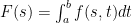 and we’d like to know what
  is.
is. .
. to make this result true: continuity of
  on some rectangle in
  space which contains all of the points in question (including the interval of integration) is sufficient.
  on some interval
  , then
  and the Mean Value Theorem.
 remind you of anything? Right; this is the fraction from the Mean Value Theorem; that is, there is some
  between
  such that

 can be made as small as desired by letting
  definition of limit that:
 which implies that

