I was in a weird situation this semester in my “applied calculus” (aka “business calculus”) class. I had an awkward amount of time left (1 week) and I still wanted to do something with Taylor polynomials, but I had nowhere near enough time to cover infinite series and power series.
So, I just went ahead and introduced it “user’s manual” style, knowing that I could justify this, if I had to (and no, I didn’t), even without series. BUT there are some drawbacks too.
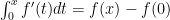
Let’s see how this goes. We’ll work with series centered at (expand about 0) and assume that has as many continuous derivatives as desired on an interval connecting 0 to .
Now we calculate: , of course. But we could do the integral another way: let’s use parts and say . Note the choice for and that is a constant in the integral. We then get . Evaluation:
and we’ve completed the first step.
Though we *could* do the inductive step now, it is useful to grind through a second iteration to see the pattern.
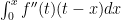
We take our expression and compute by parts again, with and insert into our previous expression:
which works out to:
and note the alternating sign of the integral.
Now to use induction: assume that:
Now let’s look at the integral: as usual, use parts as before and we obtain:
. Taking some care with the signs we end up with
which works out to .
Substituting this evaluation into our inductive step equation gives the desired result.
And note: NOTHING was a assumed except for having the required number of continuous derivatives!
BUT…yes, there is a catch. The integral is often regarded as a “correction term.” But the Taylor polynomial is really only useful so long as the integral can be made small. And that is the issue with this approach: there are times when the integral cannot be made small; it is possible that can be far enough out that the associated power series does NOT converge on and the integral picks that up, but it may well be hidden, or at least non-obvious.
And that is why, in my opinion, it is better to do series first.
Let’s show an example.
Consider . We know from work with the geometric series that its series expansion is and that the interval of convergence is But note that is smooth over and so our Taylor polynomial, with integral correction, should work for .
So, nothing that our k-th Taylor polynomial relation is:
Let’s focus on the integral; the “remainder”, if you will.
Rewrite it as: .
Now this integral really isn’t that hard to do, if we use an algebraic trick:
Rewrite
Now the integral is a simple substitutions integral: let so our integral is transformed into:
This remainder cannot be made small if no matter how big we make
But, in all honesty, this remainder could have been computed with simple algebra.
and now solve for algebraically .
The larger point is that the “error” is hidden in the integral remainder term, and this can be tough to see in the case where the associated Taylor series has a finite radius of convergence but is continuous on the whole real line, or a half line.
The problem (from Larson’s Calculus, an Applied Approach, 10’th edition, Section 7.8, no. 18 in my paperback edition, no. 17 in the e-book edition) does not seem that unusual at a very quick glance:
if you have a hard time reading the image. AND, *if* you just blindly do the formal calculations:
which is what the text has as “the answer.”
But come on. We took a function that was negative in the first quadrant, integrated it entirely in the first quadrant (in standard order) and ended up with a positive number??? I don’t think so!
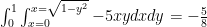
Indeed, if we perform which is far more believable.
So, we KNOW something is wrong. Now let’s attempt to sketch the region first:
Oops! Note: if we just used the quarter circle boundary we obtain
The 3-dimensional situation: we are limited by the graph of the function, the cylinder and the planes ; the plane is outside of this cylinder. (from here: the red is the graph of
Now think about what the “formal calculation” really calculated and wonder if it was just a coincidence that we got the absolute value of the integral taken over the rectangle
Let me start by saying that this is NOT: this is not an introduction for calculus students (too steep) nor is this intended for experienced calculus teachers. Nor is this a “you should teach it THIS way” or “introduce the concepts in THIS order or emphasize THESE topics”; that is for the individual teacher to decide.
Rather, this is a quick overview to help the new teacher (or for the teacher who has not taught it in a long time) decide for themselves how to go about it.
And yes, I’ll be giving a lot of opinions; disagree if you like.
What series will be used for.
Of course, infinite series have applications in probability theory (discrete density functions, expectation and higher moment values of discrete random variables), financial mathematics (perpetuities), etc. and these are great reasons to learn about them. But in calculus, these tend to be background material for power series.
Power series:, the most important thing is to determine the open interval of absolute convergence; that is, the intervals on which converges.
We teach that these intervals are *always* symmetric about (that is, at only, on some open interval or the whole real line. Side note: this is an interesting place to point out the influence that the calculus of complex variables has on real variable calculus! These open intervals are the most important aspect as one can prove that one can differentiate and integrate said series “term by term” on the open interval of absolute convergence; sometimesone can extend the results to the boundary of the interval.
Therefore, if time is limited, I tend to focus on material more relevant for series that are absolutely convergent though there are some interesting (and fun) things one can do for a series which is conditionally convergent (convergent, but not absolutely convergent; e. g. .
Important principles: I think it is a good idea to first deal with geometric series and then series with positive terms…make that “non-negative” terms.
Geometric series:; here we see that for , and is equal to for ; to show this do the old “shifted sum” addition: , then subtract: as most of the terms cancel with the subtraction.
Now to show the geometric series converges, (convergence being the standard kind: the “n’th partial sum, then the series converges if an only if the sequence of partial sums converges; yes there are other types of convergence)
Now that we’ve established that for the geometric series, and we get convergence if goes to zero, which happens only if .
Why geometric series: two of the most common series tests (root and ratio tests) involve a comparison to a geometric series. Also, the geometric series concept is used both in the theory of improper integrals and in measure theory (e. g., showing that the rational numbers have measure zero).
Series of non-negative terms. For now, we’ll assume that has all (suppressing the indices).
Main principle: though most texts talk about the various tests, I believe that most of the tests involved really involve three key principles, two of which the geometric series and the following result from sequences of positive numbers:
Key sequence result: every monotone bounded sequence of positive numbers converges to its least upper bound.
True: many calculus texts don’t do that much with the least upper bound concept but I feel it is intuitive enough to at least mention. If the least upper bound is, say, , then if is the sequence in question, there has to be some such that for any small, positive . Then because is monotone, for all
The third key principle is “common sense” : if converges (standard convergence) then as a sequence. This is pretty clear if the are non-negative; the idea is that the sequence of partial sums cannot converge to a limit unless becomes arbitrarily small. Of course, this is true even if the terms are not all positive.
Secondary results I think that the next results are “second order” results: the main results depend on these, and these depend on the key 3 that we just discussed.
The first of these secondary results is the direct comparison test for series of non-negative terms:
Direct comparison test
If and converges, then so does . If diverges, then so does .
The proof is basically the “bounded monotone sequence” principle applied to the partial sums. I like to call it “if you are taller than an NBA center then you are tall” principle.
Absolute convergence: this is the most important kind of convergence for power series as this is the type of convergence we will have on an open interval. A series is absolutely convergent if converges. Now, of course, absolute convergence implies convergence:
Note and if converges, then converges by direct comparison. Now note is the difference of two convergent series: and therefore converges.
Integral test This is an important test for convergence at a point. This test assumes that is a non-negative, non-decreasing function on some (that is, ) Then converges if and only if converges as an improper integral.
Proof: is just a right endpoint Riemann sum for and therefore the sequence of partial sums is an increasing, bounded sequence. Now if the sum converges, note that is the right endpoint estimate for so the integral can be defined as a limit of a bounded, increasing sequence so the integral converges.
Yes, these are crude whiteboards but they get the job done.
Note: we need the hypothesis that is decreasing (or non-decreasing). Example: the function certainly has converging but diverging.
Going the other way, defining gives an unbounded function with unbounded sum but the integral converges to the sum . The “boxes” get taller and skinnier.
Note: the above shows the integral and sum starting at 0; same principle though.
Now wait a minute: we haven’t really gone over how students will do most of their homework and exam problems. We’ve covered none of these: p-test, limit comparison test, ratio test, root test. Ok, logically, we have but not practically.
Let’s remedy that. First, start with the “point convergence” tests.
p-test. This says that converges if and diverges otherwise. Proof: Integral test.
Limit comparison test Given two series of positive terms: and
Suppose
If converges and then so does .
If diverges and then so does
I’ll show the “converge” part of the proof: choose then such that This means and we get convergence by direct comparison. See how useful that test is?
But note what is going on: it really isn’t necessary for to exist; for the convergence case it is only necessary that there be some for which ; if one is familiar with the limit superior (“limsup”) that is enough to make the test work.
We will see this again.
Why limit comparison is used: Something like clearly converges, but nailing down the proof with direct comparison can be hard. But a limit comparison with is pretty easy.
Ratio test this test is most commonly used when the series has powers and/or factorials in it. Basically: given consider (if the limit exists..if it doesn’t..stay tuned).
If the series converges. If the series diverges. If the test is inconclusive.
Note: if it turns out that there is exists some such that for all we have then the series converges (we can use the limsup concept here as well)
Why this works: suppose there exists some such that for all we have Then write
now factor out a to obtain
Now multiply the terms by 1 in a clever way:
See where this is going: each ratio is less than so we have:
which is a convergent geometric series.
See: there is geometric series and the direct comparison test, again.
Root Test No, this is NOT the same as the ratio test. In fact, it is a bit “stronger” than the ratio test in that the root test will work for anything the ratio test works for, but there are some series that the root test works for that the ratio test comes up empty.
I’ll state the “lim sup” version of the ratio test: if there exists some such that, for all we have then the series converges (exercise: find the “divergence version”).
As before: if the condition is met, so the original series converges by direction comparison.
Now as far as my previous remark about the ratio test: Consider the series:
Yes, this series is bounded by the convergent geometric series with and therefore converges by direct comparison. And the limsup version of the root test works as well.
But the ratio test is a disaster as which is unbounded..but .
What about non-absolute convergence (aka “conditional convergence”)
Series like converges but does NOT converge absolutely (p-test). On one hand, such series are a LOT of fun..but the convergence is very slow and unstable and so might say that these series are not as important as the series that converges absolutely. But there is a lot of interesting mathematics to be had here.
So, let’s chat about these a bit.
We say is conditionally convergent if the series converges but diverges.
One elementary tool for dealing with these is the alternating series test:
for this, let and for all .
Then converges if and only if as a sequence.
That the sequence of terms goes to zero is necessary. That it is sufficient in this alternating case: first note that the terms of the sequence of partial sums are bounded above by (as the magnitudes get steadily smaller) and below by (same reason. Note also that so the sequence of partial sums of even index are an increasing bounded sequence and therefore converges to some limit, say, . But and so by a routine “epsilon-N” argument the odd partial sums converge to as well.
Of course, there are conditionally convergent series that are NOT alternating. And conditionally convergent series have some interesting properties.
One of the most interesting properties is that such series can be “rearranged” (“derangment” in Knopp’s book) to either converge to any number of choice or to diverge to infinity or to have no limit at all.
Here is an outline of the arguments:
To rearrange a series to converge to , start with the positive terms (which must diverge as the series is conditionally convergent) and add them up to exceed ; stop just after is exceeded. Call that partial sum . Note: this could be 0 terms. Now use the negative terms to go of the left of and stop the first one past. Call that Then move to the right, past again with the positive terms..note that the overshoot is smaller as the terms are smaller. This is . Then go back again to get to the left of . Repeat.
Note that at every stage, every partial sum after the first one past is between some and the bracket and the distance is shrinking to become arbitrarily small.
To rearrange a series to diverge to infinity: Add the positive terms to exceed 1. Add a negative term. Then add the terms to exceed 2. Add a negative term. Repeat this for each positive integer .
Have fun with this; you can have the partial sums end up all over the place.
Of course, one proves the limit comparison test by the direct comparison test. But in a calculus course, the limit comparison test might appear to be more readily useful..example:
Show converges.
So..what about the direct comparison test?
As someone pointed out: the direct comparison can work very well when you don’t know much about the matrix.
One example can be found when one shows that the matrix exponential where is a matrix.
For those unfamiliar: where the powers make sense as is square and we merely add the corresponding matrix entries.
What enables convergence is the factorial in the denominators of the individual terms; the i-j’th element of each can get only so large.
But how does one prove convergence?
The usual way is to dive into matrix norms; one that works well is (just sum up the absolute value of the elements (the Taxi cab norm or norm )
Then one can show and and together this implies the following:
For any index where is the i-j’th element of we have:
It then follows that . Therefore every series that determines an entry of the matrix is an absolutely convergent series by direct comparison. and is therefore a convergent series.
The usual is to use which transforms this to the dreaded integral, which is a double integration by parts.
Is there a way out? I think so, though the price one pays is a trickier conversion back to x.
Let’s try so upon substituting we obtain and noting that alaways:
Now this can be integrated by parts: let
So but this easily reduces to:
Division by 2:
That was easy enough.
But we now have the conversion to x:
So far, so good. But what about ?
Write:
Now multiply both sides by to get and use the quadratic formula to get
We need so and that is our integral:
I guess that this isn’t that much easier after all.
The introduction is for a student who might not have seen logarithmic differentiation before: (and yes, this technique is extensively used..for example it is used in the “maximum likelihood function” calculation frequently encountered in statistics)
Suppose you are given, say, and you are told to calculate the derivative?
Calculus texts often offer the technique of logarithmic differentiation: write
Now differentiate both sides:
Now multiply both sides by to obtain
\
And this is correct…sort of. Why I say sort of: what happens, at say, ? The derivative certainly exists there but what about that second factor? Yes, the sin(x) gets cancelled out by the first factor, but AS WRITTEN, there is an oh-so-subtle problem with domains.
You can only substitute only after simplifying ..which one might see as a limit process.
But let’s stop and take a closer look at the whole process: we started with and then took the log of both sides. Where is the log defined? And when does ? You got it: this only works when .
So, on the face of it, is justified only when each .
Why can we get away with ignoring all of this, at least in this case?
Well, here is why:
1. If is a differentiable function then
Yes, this is covered in the derivation of material but here goes: write
Now if we get as usual. If then and so in either case:
as required.
THAT is the workaround for calculating where : just calculate . noting that
Yay! We are almost done! But, what about the cases where at least some of the factors are zero at, say ?
Here, we have to bite the bullet and admit that we cannot take the log of the product where any of the factors have a zero, at that point. But this is what we can prove:
Given is a product of differentiable functions and then
This works out to what we want by cancellation of factors.
Here is one way to proceed with the proof:
1. Suppose are differentiable and . Then and
2. Now suppose are differentiable and . Then and
3.Now apply the above to is a product of differentiable functions and
If then by inductive application of 1.
If then let as in 2. Then by 2, we have Now this quantity is zero unless and . But in this case note that
So there it is. Yes, it works ..with appropriate precautions.
Let’s look at an “easy” starting example: write
We know how that goes: multiply both sides by to get and then since this must be true for ALL , substitute to get and then substitute to get . Easy-peasy.
BUT…why CAN you do such a substitution since the original domain excludes ?? (and no, I don’t want to hear about residues and “poles of order 1”; this is calculus 2. )
Lets start with with the restricted domain, say
Now multiply both sides by and note that, with the restricted domain we have:
But both sides are equal on the domain and the limit on the left hand side is So the right hand side has a limit which exists and is equal to . So the result follows..and this works for the calculation for B as well.
Yes, no engineer will care about this. But THIS is the reason we can substitute the non-domain points.
As an aside: if you are trying to solve something like one can do the denominator clearing, and, as appropriate substitute and compare real and imaginary parts ..and yes, now you can use poles and residues.
My interest in “beta” functions comes from their utility in Bayesian statistics. A nice 78 minute introduction to Bayesian statistics and how the beta distribution is used can be found here; you need to understand basic mathematical statistics concepts such as “joint density”, “marginal density”, “Bayes’ Rule” and “likelihood function” to follow the youtube lecture. To follow this post, one should know the standard “3 semesters” of calculus and know what the gamma function is (the extension of the factorial function to the real numbers); previous exposure to the standard “polar coordinates” proof that would be very helpful.
So, what it the beta function? it is where . Note that for integers The gamma function is the unique “logarithmically convex” extension of the factorial function to the real line, where “logarithmically convex” means that the logarithm of the function is convex; that is, the second derivative of the log of the function is positive. Roughly speaking, this means that the function exhibits growth behavior similar to (or “greater”) than
Now it turns out that the beta density function is defined as follows: for as one can see that the integral is either proper or a convergent improper integral for .
I'll do this in two steps. Step one will convert the beta integral into an integral involving powers of sine and cosine. Step two will be to write as a product of two integrals, do a change of variables and convert to an improper integral on the first quadrant. Then I'll convert to polar coordinates to show that this integral is equal to
Step one: converting the beta integral to a sine/cosine integral. Limit and then do the substitution . Then the beta integral becomes:
Step two: transforming the product of two gamma functions into a double integral and evaluating using polar coordinates.
Write
Now do the conversion to obtain:
(there is a tiny amount of algebra involved)
From which we now obtain
Now we switch to polar coordinates, remembering the that comes from evaluating the Jacobian of
This splits into two integrals:
The first of these integrals is just so now we have:
The second integral: we just use to obtain:
(yes, I cancelled the 2 with the 1/2)
And so the result follows.
That seems complicated for a simple little integral, doesn’t it?


 if you have a hard time reading the image. AND, *if* you just blindly do the formal calculations:
 which is what the text has as “the answer.”
 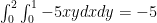 which is far more believable.
 and the planes
  ; the plane
  is outside of this cylinder. (


 find
find  That is fairly straight forward, no? But there is a bit more here than meets the eye, as I quickly found out. I graphed this on Desmos and:
 which leads to families of lines with either slope 1 or slope negative 1 and y intercepts multiples of
 which leads to:
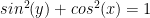
 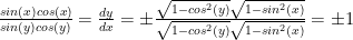 by both the original equation and the circle identity.
 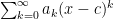 , the most important thing is to determine the open interval of absolute convergence; that is, the intervals on which
 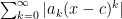 converges.
  (that is, at
  only, on some open interval
  or the whole real line. Side note: this is an interesting place to point out the influence that the calculus of complex variables has on real variable calculus! These open intervals are the most important aspect as one can prove that one can differentiate and integrate said series “term by term” on the open interval of absolute convergence; sometimes
  .
. ; here we see that for
  ,
,  and is equal to
  for
for  ; to show this do the old “shifted sum” addition:
  ,
,  then subtract:
  as most of the terms cancel with the subtraction.
  the “n’th partial sum, then the series
  converges if an only if the sequence of partial sums
  converges; yes there are
  and we get convergence if
  goes to zero, which happens only if
  .
.  has all
  (suppressing the indices).
 , then if
  is the sequence in question, there has to be some
  such that
  for any small, positive
  . Then because
  for all
 converges (standard convergence) then
  as a sequence. This is pretty clear if the
  are non-negative; the idea is that the sequence of partial sums
  becomes arbitrarily small. Of course, this is true even if the terms are not all positive.
 and
and  converges, then so does
  . If
. If  converges. Now, of course, absolute convergence implies convergence:
 and if
  converges by direct comparison. Now note
  is the difference of two convergent series:
  and therefore converges.
  (that is,
  ) Then
  converges if and only if
  converges as an improper integral.
 is just a right endpoint Riemann sum for
  is the right endpoint estimate for
 certainly has
  diverging.
![f(x) = \begin{cases} 2^n , & \text{ if } x \in [n, n+2^{-2n}] \\0, & \text{ otherwise} \end{cases}](https://s0.wp.com/latex.php?latex=f%28x%29+%3D+%5Cbegin%7Bcases%7D++2%5En+%2C+%26+%5Ctext%7B+if+%7D++x+%5Cin+%5Bn%2C+n%2B2%5E%7B-2n%7D%5D+%5C%5C0%2C+%26+%5Ctext%7B+otherwise%7D+%5Cend%7Bcases%7D+&bg=ffffff&fg=000000&s=0&c=20201002) gives an unbounded function with unbounded sum
gives an unbounded function with unbounded sum  but the integral converges to the sum
  . The “boxes” get taller and skinnier.
 converges if
  and diverges otherwise. Proof: Integral test.
 and
and 
 then so does
  then so does
  then
then  such that
  This means
  and we get convergence by direct comparison. See how useful that test is?
 to exist; for the convergence case it is only necessary that there be some
  for which
  ; if one is familiar with the
 clearly converges, but nailing down the proof with direct comparison can be hard. But a limit comparison with
  is pretty easy.
 (if the limit exists..if it doesn’t..stay tuned).
 the series converges. If
  the series diverges. If
  the test is inconclusive.
  such that for all
  we have
  then the series converges (we can use the
 to obtain
 See where this is going: each ratio is less than
  so we have:
 which is a convergent geometric series.
  we have
  then the series converges (exercise: find the “divergence version”).
  so the original series converges by direction comparison.
 and therefore converges by direct comparison. And the limsup version of the root test works as well.
  which is unbounded..but
  .
.  converges but does NOT converge absolutely (p-test). On one hand, such series are a LOT of fun..but the convergence is very slow and unstable and so might say that these series are not as important as the series that converges absolutely. But there is a lot of interesting mathematics to be had here.
 and for all
  .
. converges if and only if
  (as the magnitudes get steadily smaller) and below by
  (same reason. Note also that
  so the sequence of partial sums of even index are an increasing bounded sequence and therefore converges to some limit, say,
  . But
. But  and so by a routine “epsilon-N” argument the odd partial sums converge to
  as well.
  . Note: this could be 0 terms. Now use the negative terms to go of the left of
  Then move to the right, past
  . Then go back again to get
  to the left of
  and the
  bracket
  .
. converges.
  where
where  is a
is a  matrix.
  where the powers make sense as
  is square and we merely add the corresponding matrix entries.
  can get only so large.
 (just sum up the absolute value of the elements (the Taxi cab norm or
  and
and  and together this implies the following:
 is the i-j’th element of
![| [ e^A ]_{i,j} | \leq \sum^{\infty}_{k=0} {|A^k |\over k!} \leq \sum^{\infty}_{k=0} {|A|^k \over k!} =e^{|A|}](https://s0.wp.com/latex.php?latex=%7C+%5B+e%5EA+%5D_%7Bi%2Cj%7D+%7C+%5Cleq+%5Csum%5E%7B%5Cinfty%7D_%7Bk%3D0%7D+%7B%7CA%5Ek+%7C%5Cover+k%21%7D+%5Cleq++%5Csum%5E%7B%5Cinfty%7D_%7Bk%3D0%7D+%7B%7CA%7C%5Ek+%5Cover+k%21%7D+%3De%5E%7B%7CA%7C%7D+&bg=ffffff&fg=000000&s=0&c=20201002) . Therefore every series that determines an entry of the matrix
. Therefore every series that determines an entry of the matrix 
 which transforms this to the dreaded
  integral, which is a double integration by parts.
 so upon substituting we obtain
  and noting that
  alaways:
 Now this can be integrated by parts: let
 but this easily reduces to:


 ?
? 
 to get
  and use the quadratic formula to get
 so
so  and that is our integral:
 and you are told to calculate the derivative?

 to obtain

 ? The derivative certainly exists there but what about that second factor? Yes, the sin(x) gets cancelled out by the first factor, but AS WRITTEN, there is an oh-so-subtle problem with domains.
  only after simplifying ..which one might see as a limit process.
 and then took the log of both sides. Where is the log defined? And when does
  ? You got it: this only works when
  .
. is justified only when each
  .
. is a differentiable function then
 material but here goes: write
 we get
  as usual. If
  then
then  and so in either case:
 where
where  : just calculate
  . noting that
 ?
? is a product of differentiable functions and
 then
then
 are differentiable and
  . Then
  and
and 
 . Then
  and
and 
 then
then  by inductive application of 1.
 then let
  as in 2. Then by 2, we have
  Now this quantity is zero unless
  and
and  . But in this case note that

 to get
  and then since this must be true for ALL
  to get
  and then substitute
  to get
  . Easy-peasy.
 ?? (and no, I don’t want to hear about residues and “poles of order 1”; this is calculus 2. )
 and note that, with the restricted domain
  But both sides are equal on the domain
  and the limit on the left hand side is
  So the right hand side has a limit which exists and is equal to
  one can do the denominator clearing, and, as appropriate substitute
  and compare real and imaginary parts ..and yes, now you can use poles and residues.
  would be very helpful.
 where
where  . Note that
  for integers
  The gamma function is the unique “logarithmically convex” extension of the factorial function to the real line, where “logarithmically convex” means that the logarithm of the function is convex; that is, the second derivative of the log of the function is positive. Roughly speaking, this means that the function exhibits growth behavior similar to (or “greater”) than
 for
for  as one can see that the integral is either proper or a convergent improper integral for
  .
.  as a product of two integrals, do a change of variables and convert to an improper integral on the first quadrant. Then I'll convert to polar coordinates to show that this integral is equal to
![t \in [0, \frac{\pi}{2}]](https://s0.wp.com/latex.php?latex=t+%5Cin+%5B0%2C+%5Cfrac%7B%5Cpi%7D%7B2%7D%5D+&bg=ffffff&fg=000000&s=0&c=20201002) and then do the substitution
and then do the substitution  . Then the beta integral becomes:

 to obtain:
 (there is a tiny amount of algebra involved)
 that comes from evaluating the Jacobian of


 so now we have:
 to obtain:
 (yes, I cancelled the 2 with the 1/2)