I was in a weird situation this semester in my “applied calculus” (aka “business calculus”) class. I had an awkward amount of time left (1 week) and I still wanted to do something with Taylor polynomials, but I had nowhere near enough time to cover infinite series and power series.
So, I just went ahead and introduced it “user’s manual” style, knowing that I could justify this, if I had to (and no, I didn’t), even without series. BUT there are some drawbacks too.
Let’s see how this goes. We’ll work with series centered at (expand about 0) and assume that has as many continuous derivatives as desired on an interval connecting 0 to .
Now we calculate: , of course. But we could do the integral another way: let’s use parts and say . Note the choice for and that is a constant in the integral. We then get . Evaluation:
and we’ve completed the first step.
Though we *could* do the inductive step now, it is useful to grind through a second iteration to see the pattern.
We take our expression and compute by parts again, with and insert into our previous expression:
which works out to:
and note the alternating sign of the integral.
Now to use induction: assume that:
Now let’s look at the integral: as usual, use parts as before and we obtain:
. Taking some care with the signs we end up with
which works out to .
Substituting this evaluation into our inductive step equation gives the desired result.
And note: NOTHING was a assumed except for having the required number of continuous derivatives!
BUT…yes, there is a catch. The integral is often regarded as a “correction term.” But the Taylor polynomial is really only useful so long as the integral can be made small. And that is the issue with this approach: there are times when the integral cannot be made small; it is possible that can be far enough out that the associated power series does NOT converge on and the integral picks that up, but it may well be hidden, or at least non-obvious.
And that is why, in my opinion, it is better to do series first.
Let’s show an example.
Consider . We know from work with the geometric series that its series expansion is and that the interval of convergence is But note that is smooth over and so our Taylor polynomial, with integral correction, should work for .
So, nothing that our k-th Taylor polynomial relation is:
Let’s focus on the integral; the “remainder”, if you will.
Rewrite it as: .
Now this integral really isn’t that hard to do, if we use an algebraic trick:
Rewrite
Now the integral is a simple substitutions integral: let so our integral is transformed into:
This remainder cannot be made small if no matter how big we make
But, in all honesty, this remainder could have been computed with simple algebra.
and now solve for algebraically .
The larger point is that the “error” is hidden in the integral remainder term, and this can be tough to see in the case where the associated Taylor series has a finite radius of convergence but is continuous on the whole real line, or a half line.
This is “part 2” of a previous post about series. Once again, this is not designed for students seeing the material for the first time.
I’ll deal with general power series first, then later discuss Taylor Series (one method of obtaining a power series).
General Power Series Unless otherwise stated, we will be dealing with series such as though, of course, a series can expanded about any point in the real line (e. g. ) Note: unless it is needed, I’ll be suppressing the index in the summation sign.
So, IF we have a function ..
what do we mean by this and what can we say about it?
The first thing to consider, of course, is convergence. One main fact is that the open interval of convergence of a power series centered at 0 is either: 1. Non existent …series converges at only (e. g. ; try the ratio test) or
2. Converges absolutely on for some and diverges for all (like a geometric series) (anything possible for ) or
3. Converges absolutely on the whole real line.
Many texts state this result but do not prove it. I can understand as this result is really an artifact of calculus of a complex variable. But it won’t hurt to sketch out a proof at least for the “converge” case for so I’ll do that.
So, let’s assume that converges (either absolute OR conditional ) So, by the divergence test, we know that the sequence of terms . So we can find some index such that
So write: and converges absolutely for . The divergence follows from a simple “reversal of the inequalities (that is, if the series diverged at ).
Though the relation between real and complex variables might not be apparent, it CAN be useful. Here is an example: suppose one wants to find the open interval of convergence of, say, the series representation for ? Of course, the function itself is continuous on the whole real line. But to find the open interval of convergence, look for the complex root of that is closest to zero. That would be so the interval is
So, what about a function defined as a power series?
For one, a power series expansion of a function at a specific point (say, ) is unique:
Say on the interval of convergence, then substituting yields . So subtract from both sides and get: . Now assuming one can “factor out an x” from both sides (and you can) we get , etc.
Yes, this should have property been phrased as a limit and I’ve yet to show that is continuous on its open interval of absolute convergence.
Now if you say “doesn’t that follow from uniform convergence which follows from the Weierstrass M test” you’d be correct…and you are probably wasting your time reading this.
Now if you remember hearing those words but could use a refresher, here goes:
We want for sufficiently close AND both within the open interval of absolute convergence, say Choose where and such that and where (these are just polynomials).
The rest follows:
Calculus On the open interval of absolute convergence, a power series can be integrated term by term and differentiated term by term. Neither result, IMHO, is “obvious.” In fact, sans extra criteria, for series of functions, in general, it is false. Quickly: if you remember Fourier Series, think about the Fourier series for a rectangular pulse wave; note that the derivative is zero everywhere except for the jump points (where it is undefined), then differentiate the constituent functions and get a colossal mess.
Differentiation: most texts avoid the direct proof (with good reason; it is a mess) but it can follow from analysis results IF one first shows that the absolute (and uniform) convergence of implies the absolute (and uniform) convergence of
So, let’s start here: if is absolutely convergent on then so is .
Here is why: because we are on the open interval of absolute convergence, WLOG, assume and find where is also absolutely convergent. Now, note that so the series converges by direct comparison on which establishes what we wanted to show.
Of course, this doesn’t prove that the expected series IS the derivative; we have a bit more work to do.
Again, working on the open interval of absolute convergence, let’s look at:
Now, we use the fact that is absolutely convergent on and given any we can find so that for between and
So let’s do that: pick and then note:
Now apply the Mean Value Theorem to each term in the second term:
where each is between and . By the choice of the second term is less than , which is arbitrary, and the first term is the first terms of the “expected” derivative series.
So, THAT is “term by term” differentiation…and notice that we’ve used our hypothesis …almost all of it.
Term by term integration
Theoretically, integration combines easier with infinite summation than differentiation does. But given we’ve done differentiation, we can then do anti-differentiation by showing that converges and then differentiating.
But let’s do this independently; it is good for us. And we’ll focus on the definite integral.
(of course, )
Once again, choose so that
Then and this is less than (or equal to)
But is arbitrary and so the result follows, for definite integrals. It is an easy exercise in the Fundamental Theorem of Calculus to extract term by term anti-differentiation.
Taylor Series
Ok, now that we can say stuff about a function presented as a power series, what about finding a power series representation for a function, PROVIDED there is one? Note: we’ll need the function to have an infinite number of derivatives on an open interval about the point of expansion. We’ll also need another condition, which we will explain as we go along.
We will work with expanding about . Let be the function of interest and assume all of the relevant derivatives exist.
Start with which can be thought of as our “degree 0” expansion plus remainder term.
But now, let’s use integration by parts on the integral with (it is a clever choice for ; it just has to work.
So now we have:
It looks like we might run into sign trouble on the next iteration, but we won’t as we will see: do integration by parts again:
and so we have:
This turns out to be .
An induction argument yields
For the series to exist (and be valid over an open interval) all of the derivatives have to exist and;
.
Note: to get the Lagrange remainder formula that you see in some texts, let for and then
It is a bit trickier to get the equality as the error formula; it is a Mean Value Theorem for integrals calculation.
About the remainder term going to zero: this is necessary. Consider the classic counterexample:
It is an exercise in the limit definition and L’Hopital’s Rule to show that for all and so a Taylor expansion at zero is just the zero function, and this is valid at 0 only.
As you can see, the function appears to flatten out near x =0 $ but it really is NOT constant.
Note: of course, using the Taylor method isn’t always the best way. For example, if we were to try to get the Taylor expansion of at it is easier to use the geometric series for and substitute ; the uniqueness of the power series expansion allows for that.
Let me start by saying that this is NOT: this is not an introduction for calculus students (too steep) nor is this intended for experienced calculus teachers. Nor is this a “you should teach it THIS way” or “introduce the concepts in THIS order or emphasize THESE topics”; that is for the individual teacher to decide.
Rather, this is a quick overview to help the new teacher (or for the teacher who has not taught it in a long time) decide for themselves how to go about it.
And yes, I’ll be giving a lot of opinions; disagree if you like.
What series will be used for.
Of course, infinite series have applications in probability theory (discrete density functions, expectation and higher moment values of discrete random variables), financial mathematics (perpetuities), etc. and these are great reasons to learn about them. But in calculus, these tend to be background material for power series.
Power series:, the most important thing is to determine the open interval of absolute convergence; that is, the intervals on which converges.
We teach that these intervals are *always* symmetric about (that is, at only, on some open interval or the whole real line. Side note: this is an interesting place to point out the influence that the calculus of complex variables has on real variable calculus! These open intervals are the most important aspect as one can prove that one can differentiate and integrate said series “term by term” on the open interval of absolute convergence; sometimesone can extend the results to the boundary of the interval.
Therefore, if time is limited, I tend to focus on material more relevant for series that are absolutely convergent though there are some interesting (and fun) things one can do for a series which is conditionally convergent (convergent, but not absolutely convergent; e. g. .
Important principles: I think it is a good idea to first deal with geometric series and then series with positive terms…make that “non-negative” terms.
Geometric series:; here we see that for , and is equal to for ; to show this do the old “shifted sum” addition: , then subtract: as most of the terms cancel with the subtraction.
Now to show the geometric series converges, (convergence being the standard kind: the “n’th partial sum, then the series converges if an only if the sequence of partial sums converges; yes there are other types of convergence)
Now that we’ve established that for the geometric series, and we get convergence if goes to zero, which happens only if .
Why geometric series: two of the most common series tests (root and ratio tests) involve a comparison to a geometric series. Also, the geometric series concept is used both in the theory of improper integrals and in measure theory (e. g., showing that the rational numbers have measure zero).
Series of non-negative terms. For now, we’ll assume that has all (suppressing the indices).
Main principle: though most texts talk about the various tests, I believe that most of the tests involved really involve three key principles, two of which the geometric series and the following result from sequences of positive numbers:
Key sequence result: every monotone bounded sequence of positive numbers converges to its least upper bound.
True: many calculus texts don’t do that much with the least upper bound concept but I feel it is intuitive enough to at least mention. If the least upper bound is, say, , then if is the sequence in question, there has to be some such that for any small, positive . Then because is monotone, for all
The third key principle is “common sense” : if converges (standard convergence) then as a sequence. This is pretty clear if the are non-negative; the idea is that the sequence of partial sums cannot converge to a limit unless becomes arbitrarily small. Of course, this is true even if the terms are not all positive.
Secondary results I think that the next results are “second order” results: the main results depend on these, and these depend on the key 3 that we just discussed.
The first of these secondary results is the direct comparison test for series of non-negative terms:
Direct comparison test
If and converges, then so does . If diverges, then so does .
The proof is basically the “bounded monotone sequence” principle applied to the partial sums. I like to call it “if you are taller than an NBA center then you are tall” principle.
Absolute convergence: this is the most important kind of convergence for power series as this is the type of convergence we will have on an open interval. A series is absolutely convergent if converges. Now, of course, absolute convergence implies convergence:
Note and if converges, then converges by direct comparison. Now note is the difference of two convergent series: and therefore converges.
Integral test This is an important test for convergence at a point. This test assumes that is a non-negative, non-decreasing function on some (that is, ) Then converges if and only if converges as an improper integral.
Proof: is just a right endpoint Riemann sum for and therefore the sequence of partial sums is an increasing, bounded sequence. Now if the sum converges, note that is the right endpoint estimate for so the integral can be defined as a limit of a bounded, increasing sequence so the integral converges.
Yes, these are crude whiteboards but they get the job done.
Note: we need the hypothesis that is decreasing (or non-decreasing). Example: the function certainly has converging but diverging.
Going the other way, defining gives an unbounded function with unbounded sum but the integral converges to the sum . The “boxes” get taller and skinnier.
Note: the above shows the integral and sum starting at 0; same principle though.
Now wait a minute: we haven’t really gone over how students will do most of their homework and exam problems. We’ve covered none of these: p-test, limit comparison test, ratio test, root test. Ok, logically, we have but not practically.
Let’s remedy that. First, start with the “point convergence” tests.
p-test. This says that converges if and diverges otherwise. Proof: Integral test.
Limit comparison test Given two series of positive terms: and
Suppose
If converges and then so does .
If diverges and then so does
I’ll show the “converge” part of the proof: choose then such that This means and we get convergence by direct comparison. See how useful that test is?
But note what is going on: it really isn’t necessary for to exist; for the convergence case it is only necessary that there be some for which ; if one is familiar with the limit superior (“limsup”) that is enough to make the test work.
We will see this again.
Why limit comparison is used: Something like clearly converges, but nailing down the proof with direct comparison can be hard. But a limit comparison with is pretty easy.
Ratio test this test is most commonly used when the series has powers and/or factorials in it. Basically: given consider (if the limit exists..if it doesn’t..stay tuned).
If the series converges. If the series diverges. If the test is inconclusive.
Note: if it turns out that there is exists some such that for all we have then the series converges (we can use the limsup concept here as well)
Why this works: suppose there exists some such that for all we have Then write
now factor out a to obtain
Now multiply the terms by 1 in a clever way:
See where this is going: each ratio is less than so we have:
which is a convergent geometric series.
See: there is geometric series and the direct comparison test, again.
Root Test No, this is NOT the same as the ratio test. In fact, it is a bit “stronger” than the ratio test in that the root test will work for anything the ratio test works for, but there are some series that the root test works for that the ratio test comes up empty.
I’ll state the “lim sup” version of the ratio test: if there exists some such that, for all we have then the series converges (exercise: find the “divergence version”).
As before: if the condition is met, so the original series converges by direction comparison.
Now as far as my previous remark about the ratio test: Consider the series:
Yes, this series is bounded by the convergent geometric series with and therefore converges by direct comparison. And the limsup version of the root test works as well.
But the ratio test is a disaster as which is unbounded..but .
What about non-absolute convergence (aka “conditional convergence”)
Series like converges but does NOT converge absolutely (p-test). On one hand, such series are a LOT of fun..but the convergence is very slow and unstable and so might say that these series are not as important as the series that converges absolutely. But there is a lot of interesting mathematics to be had here.
So, let’s chat about these a bit.
We say is conditionally convergent if the series converges but diverges.
One elementary tool for dealing with these is the alternating series test:
for this, let and for all .
Then converges if and only if as a sequence.
That the sequence of terms goes to zero is necessary. That it is sufficient in this alternating case: first note that the terms of the sequence of partial sums are bounded above by (as the magnitudes get steadily smaller) and below by (same reason. Note also that so the sequence of partial sums of even index are an increasing bounded sequence and therefore converges to some limit, say, . But and so by a routine “epsilon-N” argument the odd partial sums converge to as well.
Of course, there are conditionally convergent series that are NOT alternating. And conditionally convergent series have some interesting properties.
One of the most interesting properties is that such series can be “rearranged” (“derangment” in Knopp’s book) to either converge to any number of choice or to diverge to infinity or to have no limit at all.
Here is an outline of the arguments:
To rearrange a series to converge to , start with the positive terms (which must diverge as the series is conditionally convergent) and add them up to exceed ; stop just after is exceeded. Call that partial sum . Note: this could be 0 terms. Now use the negative terms to go of the left of and stop the first one past. Call that Then move to the right, past again with the positive terms..note that the overshoot is smaller as the terms are smaller. This is . Then go back again to get to the left of . Repeat.
Note that at every stage, every partial sum after the first one past is between some and the bracket and the distance is shrinking to become arbitrarily small.
To rearrange a series to diverge to infinity: Add the positive terms to exceed 1. Add a negative term. Then add the terms to exceed 2. Add a negative term. Repeat this for each positive integer .
Have fun with this; you can have the partial sums end up all over the place.
Of course, one proves the limit comparison test by the direct comparison test. But in a calculus course, the limit comparison test might appear to be more readily useful..example:
Show converges.
So..what about the direct comparison test?
As someone pointed out: the direct comparison can work very well when you don’t know much about the matrix.
One example can be found when one shows that the matrix exponential where is a matrix.
For those unfamiliar: where the powers make sense as is square and we merely add the corresponding matrix entries.
What enables convergence is the factorial in the denominators of the individual terms; the i-j’th element of each can get only so large.
But how does one prove convergence?
The usual way is to dive into matrix norms; one that works well is (just sum up the absolute value of the elements (the Taxi cab norm or norm )
Then one can show and and together this implies the following:
For any index where is the i-j’th element of we have:
It then follows that . Therefore every series that determines an entry of the matrix is an absolutely convergent series by direct comparison. and is therefore a convergent series.
It seems as if the time faculty is expected to spend on administrative tasks is growing exponentially. In our case: we’ve had some administrative upheaval with the new people coming in to “clean things up”, thereby launching new task forces, creating more committees, etc. And this is a time suck; often more senior faculty more or less go through the motions when it comes to course preparation for the elementary courses (say: the calculus sequence, or elementary differential equations).
And so:
1. Does this harm the course quality and if so..
2. Is there any effect on the students?
I should first explain why I am thinking about this; I’ll give some specific examples from my department.
1. Some time ago, a faculty member gave a seminar in which he gave an “elementary” proof of why is non-elementary. Ok, this proof took 40-50 minutes to get through. But at the end, the professor giving the seminar exclaimed: “isn’t this lovely?” at which, another senior member (one who didn’t have a Ph. D. had had been around since the 1960’s) asked “why are you happy that yet again, we haven’t had success?” The fact that a proof that could not be expressed in terms of the usual functions by the standard field operations had been given; the whole point had eluded him. And remember, this person was in our calculus teaching line up.
2. Another time, in a less formal setting, I had mentioned that I had given a brief mention to my class that one could compute and improper integral (over the real line) of an unbounded function that that a function could have a Laplace transform. A junior faculty member who had just taught differential equations tried to inform me that only functions of exponential order could have a Laplace transform; I replied that, while many texts restricted Laplace transforms to such functions, that was not mathematically necessary (though it is a reasonable restriction for an applied first course). (briefly: imagine a function whose graph consisted of a spike of height at integer points over an interval of width and was zero elsewhere.
3. In still another case, I was talking about errors in answer keys and how, when I taught courses that I wasn’t qualified to teach (e. g. actuarial science course), it was tough for me to confidently determine when the answer key was wrong. A senior, still active research faculty member said that he found errors in an answer key..that in some cases..the interval of absolute convergence for some power series was given as a closed interval.
I was a bit taken aback; I gently reminded him that was such a series.
I know what he was confused by; there is a theorem that says that if converges (either conditionally or absolutely) for some then the series converges absolutely for all where The proof isn’t hard; note that convergence of means eventually, for some positive then compare the “tail end” of the series: use and then and compare to a convergent geometric series. Mind you, he was teaching series at the time..and yes, is a senior, research active faculty member with years and years of experience; he mentored me so many years ago.
4. Also…one time, a sharp young faculty member asked around “are there any real functions that are differentiable exactly at one point? (yes: try if is rational, if is irrational.
5. And yes, one time I had forgotten that a function could be differentiable but not be (try: at
What is the point of all of this? Even smart, active mathematicians forget stuff if they haven’t reviewed it in a while…even elementary stuff. We need time to review our courses! But…does this actually affect the students? I am almost sure that at non-elite universities such as ours, the answer is “probably not in any way that can be measured.”
Think about it. Imagine the following statements in a differential equations course:
1. “Laplace transforms exist only for functions of exponential order (false)”.
2. “We will restrict our study of Laplace transforms to functions of exponential order.”
3. “We will restrict our study of Laplace transforms to functions of exponential order but this is not mathematically necessary.”
Would students really recognize the difference between these three statements?
Yes, making these statements, with confidence, requires quite a bit of difference in preparation time. And our deans and administrators might not see any value to allowing for such preparation time as it doesn’t show up in measures of performance.
This started innocently enough; I was attempting to explain why we have to be so careful when we attempt to differentiate a power series term by term; that when one talks about infinite sums, the “sum of the derivatives” might fail to exist if the sum is infinite.
yields the “square wave” function (plus zero at the jump discontinuities)
Here I graphed to
Now the resulting function fails to even be continuous. But the resulting function is differentiable except for the points at the jump discontinuities and the derivative is zero for all but a discrete set of points.
(recall: here we have pointwise convergence; to get a differentiable limit, we need other conditions such as uniform convergence together with uniform convergence of the derivatives).
But, just for the heck of it, let’s differentiate term by term and see what we get:
It is easy to see that this result doesn’t even converge to a function of any sort.
Example: let’s see what happens at
And this repeats over and over again; no limit is possible.
Something similar happens for where are relatively prime positive integers.
But something weird is going on with this sum. I plotted the terms with
(and yes, I am using as a type of “envelope function”)
BUT…if one, say, looks at
we really aren’t getting a convergence (even at irrational multiples of ). But SOMETHING is going on!
I decided to plot to
Something is going on, though it isn’t convergence. Note: by accident, I found that the pattern falls apart when I skipped one of the terms.
This is something to think about.
I wonder: for all and we can somehow get close to for given values of by allowing enough terms…but the value of is determined by how many terms we are using (not always the same value of ).
This post is inspired by Chapter 8 of Konrad Knopp’s classic Theory and Application of Infinite Series. The title of the chapter is Divergent Series.
Notation: when I talk about a series converging, I mean “converging” in the usual sense; e. g. if and then is said to be convergent with sum .
All of this makes sense since things like limits are carefully defined. But as Knopp points out, in the “days of old”, mathematicians say these series as formal objects rather than the result of careful construction. So some of these mathematicians (like Euler) had no problem saying things like . Now this is complete nonsense by our usual modern definition. But we might note that for and note that IS in the domain of the left hand side.
So, is there a way of redefining the meaning of “infinite sum” that gives us this result, while not changing the value of convergent series (defined in the standard way)? As Knopp points out in his book, the answer is “yes” and he describes several definitions of summation that
1. Do not change the value of an infinite sum that converges in the traditional sense and
2. Allows for more series to coverge.
We’ll discuss one of these methods, commonly referred to as Cesàro summation. There are ways to generalize this.
How this came about
Consider the Euler example: . Clearly, and so this geometric series diverges. But notice that the arithmetic average of the partial sums, computed as does tend to as tends to infinity: whereas and both of these quantities tend to as tends to infinity.
So, we need to see that this method of summing is workable; that is, do infinite sums that converge in the previous sense still converge to the same number with this method?
The answer is, of course, yes. Here is how to see this: Let be a sequence that converges to zero. Then for any we can find such that implies that . So for we have Because is fixed, the first fraction tends to zero as tends to infinity. The second fraction is smaller than in absolute value. But is arbitrary, hence this arithmetic average of this null sequence is itself a null sequence.
Now let and let Now subtract note and the forms a null sequence. Then so do the .
Now to be useful, we’d have to show that series that are summable in the Cesàro obey things like the multiplicative laws; they do but I am too lazy to show that. See the Knopp book.
I will mention a couple of interesting (to me) things though. Neither is really profound.
1. If a series diverges to infinity (that is, if for any positive there exists such that for all , then this series is NOT Cesàro summable. It is relatively easy to see why: given such an then consider which is greater than for large . Hence the Cesàro partial sum becomes unbounded.
Upshot: there is no hope in making something like into a convergent series by this method. Now there is a way of making an alternating, divergent series into a convergent one via doing something like a “double Cesàro sum” (take arithmetic averages of the arithmetic averages) but that is a topic for another post.
2. Cesàro summation may speed up convergent of an alternating series which passes the alternating series test, OR it might slow it down. I’ll have to develop this idea more fully. But I invite the reader to try Cesàro summation for and on and on . In the first two cases, the series converges slowly enough so that Cesàro summation speeds up convergence. Cesàro slows down the convergence in the geometric series though. It is interesting to ponder why.
Here is the following question: start with a divergent series of positive terms which form a decreasing (non-increasing) sequence which tends to zero, say, . Now how does one select a subset of series terms to delete so as to obtain a convergent series? The Kundson article shows that one can do this with the harmonic series by, say, deleting all numbers that contain a specific digit (say, 9). I’ll talk about the proof here. But I’d like to start more basic and to bring in language used in the Ferdinands article.
So, let’s set the stage: we will let denote the divergent sum in question. All terms will be positive, for all and . Now let represent a sequence where for all ; then is called a selective sum of . I’ll call the the selecting sequence and, from the start, rule out selecting sequences that are either eventually 1 (which means that the selected series diverges since the original series did) or eventually zero (just a finite sum).
Now we’ll state a really easy result:
There is some non-eventually constant such that converges. Here is why: because , for each one can find a maximal index so that . Now select if and otherwise. Then and therefore the selected series converges by comparison with a convergent geometric series.
Of course, this result is petty lame; this technique discards a lot of terms. A cheap way to discard “fewer” terms (“fewer” meaning: in terms of “set inclusion”): Do the previous construction, but instead of using use where is a positive integer of choice. Note that
Here is an example of how this works: Consider the divergent series and the convergent geometric series Of course so but then for we have . So for . But because . The next non-zero selection coefficient is as .
Now playing with this example, we see that for but not for . So for and . So the first few are . Of course the gap between the grows as does.
Now let’s get back to the cartoon example. From this example, we’ll attempt to state a more general result.
Claim: given where if contains a 9 as one of its digits, then converges. Hint on how to prove this (without reading the solution): count the number of integers between and that lack a 9 as a digit. Then do a comparison test with a convergent geometric series, noting that every term is less than or equal to .
How to prove the claim: we can start by “counting” the number of integers between 0 and that contain no 9’s as a digit.
Between 0 and 9: clearly 0-8 inclusive, or 9 numbers.
Between 10 and 99: a moment’s thought shows that we have numbers with no 9 as a digit (hint: consider 10-19, 20-29…80-89) so this means that we have numbers between 0 and 99 with no 9 as a digit.
This leads to the conjecture: there are numbers between 0 and with no 9 as a digit and between and with no 9 as a digit.
This is verified by induction. This is true for
Assume true for . Then to find the number of numbers without a 9 between and we get which then means we have numbers between 0 and with no 9 as a digit. So our conjecture is proved by induction.
Now note that
This establishes that
So it follows that and hence our selected sum is convergent.
Further questions: ok, what is going on is that we threw out enough terms of the harmonic series for the series to converge. Between terms and we allowed terms to survive.
This suggests that if we permit up to terms between and to survive ( fixed and positive) then we will have a convergent series. I’d be interested in seeing if there is an generalization of this.
But I am tried, I have a research article to review and I need to start class preparation for the upcoming spring semester. So I’ll stop here. For now. 🙂
One thing that surprised me about the professor’s job (at a non-research intensive school; we have a modest but real research requirement, but mostly we teach): I never knew how much time I’d spend doing tasks that have nothing to do with teaching and scholarship. Groan….how much of this do I tell our applicants that arrive on campus to interview? 🙂
But there is something mathematical that I want to talk about; it is a follow up to this post. It has to do with what string theorist tell us: . Needless to say, they are using a non-standard definition of “value of a series”.
Where I think the problem is: when we hear “series” we think of something related to the usual process of addition. Clearly, this non-standard assignment doesn’t related to addition in the way we usually think about it.
So, it might make more sense to think of a “generalized series” as a map from the set of sequences of real numbers (or: the infinite dimensional real vector space) to the real numbers; the usual “limit of partial sums” definition has some nice properties with respect to sequence addition, scalar multiplication and with respect to a “shift operation” and addition, provided we restrict ourselves to a suitable collection of sequences (say, those whose traditional sum of components are absolutely convergent).
So, this “non-standard sum” can be thought of as a map where . That is a bit less offensive than calling it a “sum”. 🙂


 though, of course, a series can expanded about any point in the real line (e. g.
  ) Note: unless it is needed, I’ll be suppressing the index in the summation sign.
 ..
.. only (e. g.
  ; try the ratio test) or
  for some
  and diverges for all
  (like a geometric series) (anything possible for
  ) or
) or converges (either absolute OR conditional ) So, by the divergence test, we know that the sequence of terms
  . So we can find some index
  such that
 and
and  converges absolutely for
  . The divergence follows from a simple “reversal of the inequalities (that is, if the series diverged at
  ).
). ? Of course, the function itself is continuous on the whole real line. But to find the open interval of convergence, look for the complex root of
  that is closest to zero. That would be
  so the interval is
 ) is unique:
 on the interval of convergence, then substituting
  yields
  . So subtract from both sides and get:
  . Now assuming one can “factor out an x” from both sides (and you can) we get
  , etc.
  is continuous on its open interval of absolute convergence.
 for
for  sufficiently close AND both within the open interval of absolute convergence, say
  where
where  and
and  and
and  where
where  (these are just polynomials).


 then so is
  .
. where
where  is also absolutely convergent. Now, note that
  so the series
  converges by direct comparison on
 is absolutely convergent on
  we can find
  so that
  for
for  between
 and then note:


 where each
  is between
  the second term is less than
  , which is arbitrary, and the first term is the first
  terms of the “expected” derivative series.
 converges and then differentiating.
  (of course,
 ![[a,b] \subset (-r, r)](https://s0.wp.com/latex.php?latex=%5Ba%2Cb%5D+%5Csubset+%28-r%2C+r%29+&bg=ffffff&fg=000000&s=0&c=20201002) )
)
 and this is less than (or equal to)
 be the function of interest and assume all of the relevant derivatives exist.
  which can be thought of as our “degree 0” expansion plus remainder term.
  (it is a clever choice for
  ; it just has to work.
 and so we have:
 .
.
 .
. for
for ![t \in [0,x]](https://s0.wp.com/latex.php?latex=t+%5Cin+%5B0%2Cx%5D+&bg=ffffff&fg=000000&s=0&c=20201002) and then
and then 
 as the error formula; it is a Mean Value Theorem for integrals calculation.
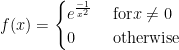
 for all
  and so a Taylor expansion at zero is just the zero function, and this is valid at 0 only.
 at
at  and substitute
  ; the uniqueness of the power series expansion allows for that.
  , the most important thing is to determine the open interval of absolute convergence; that is, the intervals on which
  converges.
  only, on some open interval
  or the whole real line. Side note: this is an interesting place to point out the influence that the calculus of complex variables has on real variable calculus! These open intervals are the most important aspect as one can prove that one can differentiate and integrate said series “term by term” on the open interval of absolute convergence; sometimes
  .
. ; here we see that for
  ,
,  and is equal to
  for
for  ; to show this do the old “shifted sum” addition:
  ,
,  then subtract:
  as most of the terms cancel with the subtraction.
  the “n’th partial sum, then the series
  converges if an only if the sequence of partial sums
  converges; yes there are
  and we get convergence if
  goes to zero, which happens only if
  .
.  has all
  (suppressing the indices).
 , then if
  is the sequence in question, there has to be some
  such that
  for any small, positive
  . Then because
  for all
 converges (standard convergence) then
  as a sequence. This is pretty clear if the
  are non-negative; the idea is that the sequence of partial sums
  becomes arbitrarily small. Of course, this is true even if the terms are not all positive.
 and
and  converges, then so does
  . If
. If  converges. Now, of course, absolute convergence implies convergence:
 and if
  converges by direct comparison. Now note
  is the difference of two convergent series:
  and therefore converges.
  (that is,
  ) Then
  converges if and only if
  converges as an improper integral.
 is just a right endpoint Riemann sum for
  is the right endpoint estimate for
 certainly has
  diverging.
![f(x) = \begin{cases} 2^n , & \text{ if } x \in [n, n+2^{-2n}] \\0, & \text{ otherwise} \end{cases}](https://s0.wp.com/latex.php?latex=f%28x%29+%3D+%5Cbegin%7Bcases%7D++2%5En+%2C+%26+%5Ctext%7B+if+%7D++x+%5Cin+%5Bn%2C+n%2B2%5E%7B-2n%7D%5D+%5C%5C0%2C+%26+%5Ctext%7B+otherwise%7D+%5Cend%7Bcases%7D+&bg=ffffff&fg=000000&s=0&c=20201002) gives an unbounded function with unbounded sum
gives an unbounded function with unbounded sum  but the integral converges to the sum
  . The “boxes” get taller and skinnier.
 converges if
  and diverges otherwise. Proof: Integral test.
 and
and 
 then so does
  then so does
  then
then  such that
  This means
  and we get convergence by direct comparison. See how useful that test is?
 to exist; for the convergence case it is only necessary that there be some
  ; if one is familiar with the
 clearly converges, but nailing down the proof with direct comparison can be hard. But a limit comparison with
  is pretty easy.
 (if the limit exists..if it doesn’t..stay tuned).
 the series converges. If
  the series diverges. If
  the test is inconclusive.
  such that for all
  we have
  then the series converges (we can use the
 to obtain
 See where this is going: each ratio is less than
  so we have:
 which is a convergent geometric series.
  we have
  then the series converges (exercise: find the “divergence version”).
  so the original series converges by direction comparison.
 and therefore converges by direct comparison. And the limsup version of the root test works as well.
  which is unbounded..but
  .
.  converges but does NOT converge absolutely (p-test). On one hand, such series are a LOT of fun..but the convergence is very slow and unstable and so might say that these series are not as important as the series that converges absolutely. But there is a lot of interesting mathematics to be had here.
 and for all
  .
. converges if and only if
  (as the magnitudes get steadily smaller) and below by
  (same reason. Note also that
  so the sequence of partial sums of even index are an increasing bounded sequence and therefore converges to some limit, say,
  . But
. But  and so by a routine “epsilon-N” argument the odd partial sums converge to
  as well.
  . Note: this could be 0 terms. Now use the negative terms to go of the left of
  Then move to the right, past
  . Then go back again to get
  to the left of
  and the
  bracket
  converges.
  where
where  is a
is a  matrix.
  where the powers make sense as
  is square and we merely add the corresponding matrix entries.
  can get only so large.
 (just sum up the absolute value of the elements (the Taxi cab norm or
  and
and  and together this implies the following:
 is the i-j’th element of
![| [ e^A ]_{i,j} | \leq \sum^{\infty}_{k=0} {|A^k |\over k!} \leq \sum^{\infty}_{k=0} {|A|^k \over k!} =e^{|A|}](https://s0.wp.com/latex.php?latex=%7C+%5B+e%5EA+%5D_%7Bi%2Cj%7D+%7C+%5Cleq+%5Csum%5E%7B%5Cinfty%7D_%7Bk%3D0%7D+%7B%7CA%5Ek+%7C%5Cover+k%21%7D+%5Cleq++%5Csum%5E%7B%5Cinfty%7D_%7Bk%3D0%7D+%7B%7CA%7C%5Ek+%5Cover+k%21%7D+%3De%5E%7B%7CA%7C%7D+&bg=ffffff&fg=000000&s=0&c=20201002) . Therefore every series that determines an entry of the matrix
. Therefore every series that determines an entry of the matrix  is
is  at integer points over an interval of width
  and was zero elsewhere.
  was such a series.
  converges (either conditionally or absolutely) for some
  then the series converges absolutely for all
  where
where  The proof isn’t hard; note that convergence of
  for some positive
  and then
  and compare to a convergent geometric series. Mind you, he was teaching series at the time..and yes, is a senior, research active faculty member with years and years of experience; he mentored me so many years ago.
 if
if  if
if  (try:
(try:  at
at 
 yields the “square wave” function (plus zero at the jump discontinuities)


 where
where  are relatively prime positive integers.

 as a type of “envelope function”)

 ). But SOMETHING is going on!

 and we can somehow get close to
  for given values of
  and
and  then
then  is said to be convergent with sum
  . Now this is complete nonsense by our usual modern definition. But we might note that
  for
for  and note that
  IS in the domain of the left hand side.
  . Clearly,
  and so this geometric series diverges. But notice that the arithmetic average of the partial sums, computed as
  does tend to
  as
as  whereas
  and both of these quantities tend to
  be a sequence that converges to zero. Then for any
  implies that
  . So for
  we have
  Because
  and let
  Now subtract note
  and the
  forms a null sequence. Then so do the
  .
. , then this series is NOT Cesàro summable. It is relatively easy to see why: given such an
  then consider
  which is greater than
  for large
  into a convergent series by this method. Now there is a way of making an alternating, divergent series into a convergent one via doing something like a “double Cesàro sum” (take arithmetic averages of the arithmetic averages) but that is a topic for another post.
 and on
  and on
  . In the first two cases, the series converges slowly enough so that Cesàro summation speeds up convergence. Cesàro slows down the convergence in the geometric series though. It is interesting to ponder why.
 . Now how does one select a subset of series terms to delete so as to obtain a convergent series? The Kundson article shows that one can do this with the harmonic series by, say, deleting all numbers that contain a specific digit (say, 9). I’ll talk about the proof here. But I’d like to start more basic and to bring in language used in the Ferdinands article.
 for all
  . Now let
  for all
  is called a selective sum of
  one can find a maximal index
  so that
  . Now select
  if
if  and
and  otherwise. Then
  and therefore the selected series converges by comparison with a convergent geometric series.
  where
where 
 and the convergent geometric series
  Of course
  so
so  but then for
  we have
  . So
. So  . But
. But  because
  . The next non-zero selection coefficient is
  as
as  .
. for
for  but not for
  . So
. So  for
for  and
and  . So the first few
  are
are  . Of course the gap between the
  where
where  and
and  that lack a 9 as a digit. Then do a comparison test with a convergent geometric series, noting that every term
  is less than or equal to
  .
. numbers with no 9 as a digit (hint: consider 10-19, 20-29…80-89) so this means that we have
  numbers between 0 and 99 with no 9 as a digit.
  numbers between 0 and
  with no 9 as a digit and
  between
  and
and  with no 9 as a digit.
 . Then to find the number of numbers without a 9 between
  and
and  we get
  which then means we have
  numbers between 0 and
  with no 9 as a digit. So our conjecture is proved by induction.


 and hence our selected sum is convergent.
  we allowed
  terms to survive.
  terms between
  to survive (
 fixed and positive) then we will have a convergent series. I’d be interested in seeing if there is an generalization of this.
  for all
  for all
 .
.  to see the series diverges.
  . Needless to say, they are using a non-standard definition of “value of a series”.
 where
where  . That is a bit less offensive than calling it a “sum”. 🙂