This might seem like a strange topic but right now our topology class is studying compact metric spaces. One of the more famous of these is the “Cantor set” or “Cantor space”. I discussed the basics of these here.
Now if you know the relationship between a countable product of two point discrete spaces (in the product topology) and Cantor spaces/Cantor Sets, this post is probably too elementary for you.
Construction: start with a two point set  and give it the discrete topology. The reason for choosing 0 and 2 to represent the elements will become clear later. Of course,
  is a compact metric space (with the discrete metric:
  if
if  .
.
Now consider the infinite product of such spaces with the product topology:  where each
  is homeomorphic to
  . It follows from the Tychonoff Theorem that
  is compact, though we can prove this directly: Let
  be any open cover for . Then choose an arbitrary
  from this open cover; because we are using the product topology
  where each
  is a one or two point set. This means that the cardinality of
  is at most
  which requires at most elements of the open cover to cover.
Now let’s examine some properties.
Clearly the space is Hausdorff ( ) and uncountable.
1. Every point of is a limit point of . To see this: denote  by the sequence
  where
where  . Then any open set containing
  is
is  and contains ALL points
  where
where  for
for  . So all points of are accumulation points of ; in fact they are condensation points (or perfect limit points ).
(refresher: accumulation points are those for which every open neighborhood contains an infinite number of points of the set in question; condensation points contain an uncountable number of points, and perfect limit points are those for which every open neighborhood contains as many points as the set in question has (same cardinality).
2. is totally disconnected (the components are one point sets). Here is how we will show this: given  there exists disjoint open sets
  . Proof of claim: if there exists a first coordinate
  for which
  (that is, a first for which the canonical projection maps disagree (
 ). Then
 ,
,

are the required disjoint open sets whose union is all of .
3. is countable, as basis elements for open sets consist of finite sequences of 0’s and 2’s followed by an infinite product of .
4. is metrizable as well;  . Note that is metric is well defined. Suppose . Then there is a first
  . Then note

which is impossible.
5. By construction is uncountable, though this follows from the fact that is compact, Haudorff and dense in itself.
6.  is homeomorphic to . The homeomorphism is given by
  . It follows that is homeomorphic to a finite product with itself (product topology). Here we use the fact that if
  is a continuous bijection with
  compact and
  Hausdorff then
  is a homeomorphism.
Now we can say a bit more: if  is a copy of then
  is homeomorphic to . This will follow from subsequent work, but we can prove this right now, provided we review some basic facts about countable products and counting.
First lets show that there is a bijection between  and
and  . A bijection is suggested by this diagram:

which has the following formula (coming up with it is fun; it uses the fact that  :
:
 for even
 for odd
 for odd,
 for even,
Here is a different bijection; it is a fun exercise to come up with the relevant formulas:

Now lets give the map between  and . Let
  and denote the elements of by
  where
where  .
.
We now describe a map  by
by

Example: 
That this is a bijection between compact Hausdorff spaces is immediate. If we show that  is continuous, we will have shown that is a homeomorphism.
But that isn’t hard to do. Let  be open;
  . Then there is some
  for which
  . Then if
  denotes the
  component of we wee that for all
  (these are entries on or below the diagonal containing
  depending on whether is even or odd.
So  is of the form
  where each
  is open in
  . This is an open set in the product topology of so this shows that is continuous. Therefore is a homeomorphism, therefore so is
  .
.
Ok, what does this have to do with Cantor Sets and Cantor Spaces?
If you know what the “middle thirds” Cantor Set is I urge you stop reading now and prove that that Cantor set is indeed homeomorphic to as we have described it. I’ll give this quote from Willard, page 121 (Hardback edition), section 17.9 in Chapter 6:
The proof is left as an exercise. You should do it if you think you can’t, since it will teach you a lot about product spaces.
What I will do I’ll give a geometric description of a Cantor set and show that this description, which easily includes the “deleted interval” Cantor sets that are used in analysis courses, is homeomorphic to .
Set up
I’ll call this set  and describe it as follows:
 (for those interested in the topology of manifolds this poses no restrictions since any manifold embeds in
  for sufficiently high
  ).
).
Reminder: the diameter of a set will be 
Let  be a strictly decreasing sequence of positive real numbers such that
  .
.
Let  be some closed n-ball in (that is,
  is a subset homeomorphic to a closed n-ball; we will use that convention throughout)
Let  be two disjoint closed n-balls in the interior of , each of which has diameter less than
  .
.

Let  be disjoint closed n-balls in the interior
  and
and  be disjoint closed n-balls in the interior of
  , each of which (all 4 balls) have diameter less that
  . Let
. Let 

To describe the construction inductively we will use a bit of notation:  for all
  and
and  will represent an infinite sequence of such
  .
.
Now if  has been defined, we let
  and
and  be disjoint closed n-balls of diameter less than
  which lie in the interior of
  . Note that
  consists of
  disjoint closed n-balls.
Now let  . Since these are compact sets with the finite intersection property (
 for all
  ), is non empty and compact. Now for any choice of sequence we have
  is nonempty by the finite intersection property. On the other hand, if
  then
then  so choose
  such that
  . Then
  lie in different components of
  since the diameters of these components are less than .
Then we can say that the  uniquely define the points of . We can call such points
Note: in the subspace topology, the  are open sets, as well as being closed.
Finding a homeomorphism from to .
Let  be defined by
  . This is a bijection. To show continuity: consider the open set
  . Under this pulls back to the open set (in the subspace topology)
  hence is continuous. Because is compact and is Hausdorff, is a homeomorphism.
This ends part I.
We have shown that the Cantor sets defined geometrically and defined via “deleted intervals” are homeomorphic to . What we have not shown is the following:
Let be a compact Hausdorff space which is dense in itself (every point is a limit point) and totally disconnected (components are one point sets). Then is homeomorphic to . That will be part II.


![t \in [0, \frac{\pi}{2}]](https://s0.wp.com/latex.php?latex=t+%5Cin+%5B0%2C+%5Cfrac%7B%5Cpi%7D%7B2%7D%5D+&bg=ffffff&fg=000000&s=0&c=20201002)


 centered at
  which converges on the punctured disk
  . And yes, about half the class missed it.
 and evaluate the latter integral as follows:
 (this follows from restricting
  to the unit circle
  and setting
  and then obtaining a rational function of
  And then the integral is transformed to:
 which means
  but only the roots
  lie inside the unit circle.

 and
and 
 so by Cauchy’s theorem
 and divide by two but instead just went with:
 where
where  is the upper half of
  ? Well,
  has a primitive away from those poles so isn’t this just
  , right?
  because the integrand is an odd function?
  taken in the standard direction and
  if you do this property (hint: set
 ![z(t) = e^{it}, dz = ie^{it}, t \in [0, \pi]](https://s0.wp.com/latex.php?latex=z%28t%29+%3D+e%5E%7Bit%7D%2C+dz+%3D+ie%5E%7Bit%7D%2C+t+%5Cin+%5B0%2C+%5Cpi%5D+&bg=ffffff&fg=000000&s=0&c=20201002) . Now attempt to integrate from 1 to -1 along the real axis. What goes wrong? What goes wrong is exactly what I missed in the above example.
. Now attempt to integrate from 1 to -1 along the real axis. What goes wrong? What goes wrong is exactly what I missed in the above example. 
 yields the “square wave” function (plus zero at the jump discontinuities)


 where
where  are relatively prime positive integers.

 as a type of “envelope function”)

 ). But SOMETHING is going on!

 and we can somehow get close to
  for given values of
  by allowing enough terms…but the value of
  ,
,  , square roots, etc.
 then it is reasonable to conclude that
  . It is as if we want students to think that functions take integers to integers.
  Now consider the following covering of the rational numbers:
  . The length of each open interval is
  . Of course there will be overlapping intervals but that isn’t important. What is important is that if one sums the lengths one gets
  . So the rationals can be covered by a collection of open sets whose total length is less than or equal to 2.
  and the total length is now less than or equal to
  where
where  is any real number. Since there is no positive lower bound as to how small
 ![f: [0,1] \rightarrow [0,1] \times [0,1] \subset R^2](https://s0.wp.com/latex.php?latex=f%3A+%5B0%2C1%5D+%5Crightarrow+%5B0%2C1%5D+%5Ctimes+%5B0%2C1%5D+%5Csubset+R%5E2+&bg=ffffff&fg=000000&s=0&c=20201002) .
.![f: [0,1] \rightarrow M](https://s0.wp.com/latex.php?latex=f%3A+%5B0%2C1%5D+%5Crightarrow+M+&bg=ffffff&fg=000000&s=0&c=20201002) where
where  is, say, a manifold (a 2’nd countable metric space which has neighborhoods either locally homeomorphic to
  or
or  . Note: though we often think of smooth or piecewise linear curves, we don’t have to do so. Also, we can allow for self-intersections.
 ![f: [0,1] \rightarrow [0,1] \times [0,1]](https://s0.wp.com/latex.php?latex=f%3A+%5B0%2C1%5D+%5Crightarrow+%5B0%2C1%5D+%5Ctimes+%5B0%2C1%5D+&bg=ffffff&fg=000000&s=0&c=20201002) ; such a gadget is called a space filling curve.
; such a gadget is called a space filling curve. and
and  then
then  is said to be convergent with sum
  .
. . Now this is complete nonsense by our usual modern definition. But we might note that
  for
for  and note that
  IS in the domain of the left hand side.
  . Clearly,
  and so this geometric series diverges. But notice that the arithmetic average of the partial sums, computed as
  does tend to
  as
as  whereas
  and both of these quantities tend to
  be a sequence that converges to zero. Then for any
  we can find
  implies that
  . So for
  we have
  Because
  and let
  Now subtract note
  and the
  forms a null sequence. Then so do the
  .
. , then this series is NOT Cesàro summable. It is relatively easy to see why: given such an
  then consider
  which is greater than
  for large
  into a convergent series by this method. Now there is a way of making an alternating, divergent series into a convergent one via doing something like a “double Cesàro sum” (take arithmetic averages of the arithmetic averages) but that is a topic for another post.
 and on
  and on
  . In the first two cases, the series converges slowly enough so that Cesàro summation speeds up convergence. Cesàro slows down the convergence in the geometric series though. It is interesting to ponder why.
 we will start with the assumption that
  ; that is, the distance between the endpoints of
 ![[-R,R]](https://s0.wp.com/latex.php?latex=%5B-R%2CR%5D+&bg=ffffff&fg=000000&s=0&c=20201002) is
is  .
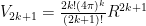
. where
where  is a constant and
  is the radius.
  hence the induction hypothesis holds for the first case and
  . We now go to show the second case because, for the beginner, the technique will be easier to follow further along if we do the
  case.
case. and you’ve seen many demonstrations of this fact. Here is another: let’s calculate this using the method of “area by cross sections”. Here is
  with some
  cross sections drawn in.
 level, call the radius from the center line to the circle
  so the total length of the “y is constant” level is
  and we “multiply by thickness “dy” to obtain
  .
.  we have
  and so our integral is
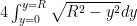
 to change the integral to:
 therefore
  where:

 as expected.
 and
and  by using the above methods.
 Now calculate using the method of cross sections above (and here we move away from x-y coordinates to more general labeling):
 and so
  . Now for the key observation:
  and so

 and the integral is now:
 which is what we needed to show.
 and, in general,
 is useful (it is merely integration by parts). Now use the limits and elementary calculation to obtain:
 to obtain:
 if
if  if
if  .
.  and see how it holds up:

 factor. All factors cancel except for the
  in the first denominator and the 2 in the first numerator, as well as the
  factor. This leads to:
 as required.

 in the denominator and put one between each denominator factor:
 Now multiply the denominator by
  and put one factor with each
  factor in the denominator; also multiply by
  Now gather each factor of 2 in the numerator product of the 2k, 2k-2…
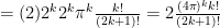 which is the required formula.
 . If this seems strange at first, think of it this way: imagine the n-ball being “inscribed” in an n-cube which has hyper volume
  . Then consider the ratio
  ; that is, the n-ball holds a smaller and smaller percentage of the hyper volume of the n-cube that it is inscribed in; note the
  corresponds to the number of corners in the n-cube. One might see that the rounding gets more severe as the number of dimensions increases.
 as well.


