But: it is no secret that higher education in the US is in turmoil, at least at the non-elite universities. Some colleges are closing and others are experiencing cut backs due to high operating losses.
This little not will not attempt to explain the problems of why education has gotten so expensive, though things like: reduction of government subsidies, increased costs for technology (computers, wifi, learning management systems), unfunded mandates (e. g. accommodations for an increasing percentage of students with learning disabilities) and staff to handle helicopter parents are all factors adding to increased costs.
And so, many universities are more tuition dependent than ever before, and while the sticker price is high, many (most in many universities) are given steep discounts.
And so, higher administration is trying to figure out what to offer: they need to bring in tuition dollars.
Now about math: our number of majors has dropped, and much, if not most, of the drop comes from math education: teaching is not a popular occupation right now, for many reasons.
Things like this do not help attract student to teacher education programs:
Virginia argues teacher is not entitled to extra compensation after being shot because the shooting was a "hazard of the job." The school board's attorney says it's an "unfortunate reality" that teaching is "not without its dangers."https://t.co/t3H7Sf70dz
One thing that hurts enrollment in upper division math courses is that higher math has prerequisites. Of course, many (most?) pure math courses do not appear to have immediate application to other fields (though they often do). And, let’s face it: math is hard. The ideas are very dense.
So, it is my feeling that the math major..one that requires two semesters of abstract algebra and two semesters of analysis, is probably on the way out, at least at non-elite schools. I think it will survive at Ivy caliber schools, MIT, Stanford, and the flagship R-1 schools.
As far as the rest of us: it absolutely hurts my heart to say this, but I feel that for our major to survive at a place like mine, we’ll have to allow for at least some upper division credit to come from “theory of interest”, “math for data science”, etc. type courses…and perhaps allow for mathy electives from other disciplines. I see us as having to become a “mathematical sciences” type program…or not existing at all.
Now for the West Virginia situation (and they probably won’t be the last):
I went on their faculty page and noted that they had 31 Associate/Full professors; the remainder appeard to be “instructors” or “assistant professors of instruction” and the like. So while I do not have any special information, it appears that they are cutting the non-tenured..the ones who did a lot (most?) of the undergraduate teaching.
Now for the uninitiated: keeping current with research at the R-1 level is, in and of itself, is a full time job. Now I am NOT one of those who says that “researchers are bad teachers” (that is often untrue) but I can say that teaching full loads (10-12 hours of undergraduate classes) is a very different job than running a graduate seminar, advising graduate students, researching, and getting NSF grants (often a prerequisite for getting tenure to begin with.
So, a lot of professor’s lives are going to change, not only for those being let go, but also for those still left. I’d imagine that some of the research professors might leave and have their place taken by the teaching faculty who are due to be cut, but that is pure speculation on my part.
This caught my eye. Pay attention to how the professor responds.
.@Riley_Gaines_ to anthropologist: "If you were to dig up… 2 humans… 100 years from now, both man and woman, could you tell the difference, strictly off of bones?"
"No."
*CHAOS*
"I'm not sure why I'm being laughed at if I'm the expert in the room. … I have a PhD!" pic.twitter.com/YYW76ISevI
He seemed genuinely rattled at being laughed at in public. And notice how he responded with “Hey, I am the expert here!”
I wonder if he has a lot of experience teaching courses in which many of the students really don’t want to be there, but have to be.
And that is what I have learned from teaching such courses: if you are going to given an answer that seems to go against the “common sense” of the student, it is a good thing to have a ready made reply such as “I can see why you might think that, but here is where it goes wrong…”
I don’t want to get too much into the details because this is a math teaching blog, not a biology blog. But it appears to me that he might have said “ok, in many cases, you can tell, but not in every case, and this is why…”
But instead, the professor pulled the “credentials card.”
Having some experience with a, well, disinterested audience (if not outright hostile at times) can be a good thing.
The problem (from Larson’s Calculus, an Applied Approach, 10’th edition, Section 7.8, no. 18 in my paperback edition, no. 17 in the e-book edition) does not seem that unusual at a very quick glance:
if you have a hard time reading the image. AND, *if* you just blindly do the formal calculations:
which is what the text has as “the answer.”
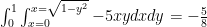
But come on. We took a function that was negative in the first quadrant, integrated it entirely in the first quadrant (in standard order) and ended up with a positive number??? I don’t think so!
Indeed, if we perform which is far more believable.
So, we KNOW something is wrong. Now let’s attempt to sketch the region first:
Oops! Note: if we just used the quarter circle boundary we obtain
The 3-dimensional situation: we are limited by the graph of the function, the cylinder and the planes ; the plane is outside of this cylinder. (from here: the red is the graph of
Now think about what the “formal calculation” really calculated and wonder if it was just a coincidence that we got the absolute value of the integral taken over the rectangle
Let me start by saying that this is NOT: this is not an introduction for calculus students (too steep) nor is this intended for experienced calculus teachers. Nor is this a “you should teach it THIS way” or “introduce the concepts in THIS order or emphasize THESE topics”; that is for the individual teacher to decide.
Rather, this is a quick overview to help the new teacher (or for the teacher who has not taught it in a long time) decide for themselves how to go about it.
And yes, I’ll be giving a lot of opinions; disagree if you like.
What series will be used for.
Of course, infinite series have applications in probability theory (discrete density functions, expectation and higher moment values of discrete random variables), financial mathematics (perpetuities), etc. and these are great reasons to learn about them. But in calculus, these tend to be background material for power series.
Power series:, the most important thing is to determine the open interval of absolute convergence; that is, the intervals on which converges.
We teach that these intervals are *always* symmetric about (that is, at only, on some open interval or the whole real line. Side note: this is an interesting place to point out the influence that the calculus of complex variables has on real variable calculus! These open intervals are the most important aspect as one can prove that one can differentiate and integrate said series “term by term” on the open interval of absolute convergence; sometimesone can extend the results to the boundary of the interval.
Therefore, if time is limited, I tend to focus on material more relevant for series that are absolutely convergent though there are some interesting (and fun) things one can do for a series which is conditionally convergent (convergent, but not absolutely convergent; e. g. .
Important principles: I think it is a good idea to first deal with geometric series and then series with positive terms…make that “non-negative” terms.
Geometric series:; here we see that for , and is equal to for ; to show this do the old “shifted sum” addition: , then subtract: as most of the terms cancel with the subtraction.
Now to show the geometric series converges, (convergence being the standard kind: the “n’th partial sum, then the series converges if an only if the sequence of partial sums converges; yes there are other types of convergence)
Now that we’ve established that for the geometric series, and we get convergence if goes to zero, which happens only if .
Why geometric series: two of the most common series tests (root and ratio tests) involve a comparison to a geometric series. Also, the geometric series concept is used both in the theory of improper integrals and in measure theory (e. g., showing that the rational numbers have measure zero).
Series of non-negative terms. For now, we’ll assume that has all (suppressing the indices).
Main principle: though most texts talk about the various tests, I believe that most of the tests involved really involve three key principles, two of which the geometric series and the following result from sequences of positive numbers:
Key sequence result: every monotone bounded sequence of positive numbers converges to its least upper bound.
True: many calculus texts don’t do that much with the least upper bound concept but I feel it is intuitive enough to at least mention. If the least upper bound is, say, , then if is the sequence in question, there has to be some such that for any small, positive . Then because is monotone, for all
The third key principle is “common sense” : if converges (standard convergence) then as a sequence. This is pretty clear if the are non-negative; the idea is that the sequence of partial sums cannot converge to a limit unless becomes arbitrarily small. Of course, this is true even if the terms are not all positive.
Secondary results I think that the next results are “second order” results: the main results depend on these, and these depend on the key 3 that we just discussed.
The first of these secondary results is the direct comparison test for series of non-negative terms:
Direct comparison test
If and converges, then so does . If diverges, then so does .
The proof is basically the “bounded monotone sequence” principle applied to the partial sums. I like to call it “if you are taller than an NBA center then you are tall” principle.
Absolute convergence: this is the most important kind of convergence for power series as this is the type of convergence we will have on an open interval. A series is absolutely convergent if converges. Now, of course, absolute convergence implies convergence:
Note and if converges, then converges by direct comparison. Now note is the difference of two convergent series: and therefore converges.
Integral test This is an important test for convergence at a point. This test assumes that is a non-negative, non-decreasing function on some (that is, ) Then converges if and only if converges as an improper integral.
Proof: is just a right endpoint Riemann sum for and therefore the sequence of partial sums is an increasing, bounded sequence. Now if the sum converges, note that is the right endpoint estimate for so the integral can be defined as a limit of a bounded, increasing sequence so the integral converges.
Yes, these are crude whiteboards but they get the job done.
Note: we need the hypothesis that is decreasing (or non-decreasing). Example: the function certainly has converging but diverging.
Going the other way, defining gives an unbounded function with unbounded sum but the integral converges to the sum . The “boxes” get taller and skinnier.
Note: the above shows the integral and sum starting at 0; same principle though.
Now wait a minute: we haven’t really gone over how students will do most of their homework and exam problems. We’ve covered none of these: p-test, limit comparison test, ratio test, root test. Ok, logically, we have but not practically.
Let’s remedy that. First, start with the “point convergence” tests.
p-test. This says that converges if and diverges otherwise. Proof: Integral test.
Limit comparison test Given two series of positive terms: and
Suppose
If converges and then so does .
If diverges and then so does
I’ll show the “converge” part of the proof: choose then such that This means and we get convergence by direct comparison. See how useful that test is?
But note what is going on: it really isn’t necessary for to exist; for the convergence case it is only necessary that there be some for which ; if one is familiar with the limit superior (“limsup”) that is enough to make the test work.
We will see this again.
Why limit comparison is used: Something like clearly converges, but nailing down the proof with direct comparison can be hard. But a limit comparison with is pretty easy.
Ratio test this test is most commonly used when the series has powers and/or factorials in it. Basically: given consider (if the limit exists..if it doesn’t..stay tuned).
If the series converges. If the series diverges. If the test is inconclusive.
Note: if it turns out that there is exists some such that for all we have then the series converges (we can use the limsup concept here as well)
Why this works: suppose there exists some such that for all we have Then write
now factor out a to obtain
Now multiply the terms by 1 in a clever way:
See where this is going: each ratio is less than so we have:
which is a convergent geometric series.
See: there is geometric series and the direct comparison test, again.
Root Test No, this is NOT the same as the ratio test. In fact, it is a bit “stronger” than the ratio test in that the root test will work for anything the ratio test works for, but there are some series that the root test works for that the ratio test comes up empty.
I’ll state the “lim sup” version of the ratio test: if there exists some such that, for all we have then the series converges (exercise: find the “divergence version”).
As before: if the condition is met, so the original series converges by direction comparison.
Now as far as my previous remark about the ratio test: Consider the series:
Yes, this series is bounded by the convergent geometric series with and therefore converges by direct comparison. And the limsup version of the root test works as well.
But the ratio test is a disaster as which is unbounded..but .
What about non-absolute convergence (aka “conditional convergence”)
Series like converges but does NOT converge absolutely (p-test). On one hand, such series are a LOT of fun..but the convergence is very slow and unstable and so might say that these series are not as important as the series that converges absolutely. But there is a lot of interesting mathematics to be had here.
So, let’s chat about these a bit.
We say is conditionally convergent if the series converges but diverges.
One elementary tool for dealing with these is the alternating series test:
for this, let and for all .
Then converges if and only if as a sequence.
That the sequence of terms goes to zero is necessary. That it is sufficient in this alternating case: first note that the terms of the sequence of partial sums are bounded above by (as the magnitudes get steadily smaller) and below by (same reason. Note also that so the sequence of partial sums of even index are an increasing bounded sequence and therefore converges to some limit, say, . But and so by a routine “epsilon-N” argument the odd partial sums converge to as well.
Of course, there are conditionally convergent series that are NOT alternating. And conditionally convergent series have some interesting properties.
One of the most interesting properties is that such series can be “rearranged” (“derangment” in Knopp’s book) to either converge to any number of choice or to diverge to infinity or to have no limit at all.
Here is an outline of the arguments:
To rearrange a series to converge to , start with the positive terms (which must diverge as the series is conditionally convergent) and add them up to exceed ; stop just after is exceeded. Call that partial sum . Note: this could be 0 terms. Now use the negative terms to go of the left of and stop the first one past. Call that Then move to the right, past again with the positive terms..note that the overshoot is smaller as the terms are smaller. This is . Then go back again to get to the left of . Repeat.
Note that at every stage, every partial sum after the first one past is between some and the bracket and the distance is shrinking to become arbitrarily small.
To rearrange a series to diverge to infinity: Add the positive terms to exceed 1. Add a negative term. Then add the terms to exceed 2. Add a negative term. Repeat this for each positive integer .
Have fun with this; you can have the partial sums end up all over the place.
Since I am online, I decided to use Webassign for homework.
Well, of course, some students have had trouble with it..in particular the graphing application.
I am not saying that their graphing tool is hard to learn; in fact I might play with it myself. BUT, in this particular class, I want my students to focus on learning the material and NOT have to spend hours learning to get good with their graphing tools. For graphing: Desmos is outstanding.
Normally, I am not sympathetic to student complaints or frustrations, but here, I can see it.
The introduction is for a student who might not have seen logarithmic differentiation before: (and yes, this technique is extensively used..for example it is used in the “maximum likelihood function” calculation frequently encountered in statistics)
Suppose you are given, say, and you are told to calculate the derivative?
Calculus texts often offer the technique of logarithmic differentiation: write
Now differentiate both sides:
Now multiply both sides by to obtain
\
And this is correct…sort of. Why I say sort of: what happens, at say, ? The derivative certainly exists there but what about that second factor? Yes, the sin(x) gets cancelled out by the first factor, but AS WRITTEN, there is an oh-so-subtle problem with domains.
You can only substitute only after simplifying ..which one might see as a limit process.
But let’s stop and take a closer look at the whole process: we started with and then took the log of both sides. Where is the log defined? And when does ? You got it: this only works when .
So, on the face of it, is justified only when each .
Why can we get away with ignoring all of this, at least in this case?
Well, here is why:
1. If is a differentiable function then
Yes, this is covered in the derivation of material but here goes: write
Now if we get as usual. If then and so in either case:
as required.
THAT is the workaround for calculating where : just calculate . noting that
Yay! We are almost done! But, what about the cases where at least some of the factors are zero at, say ?
Here, we have to bite the bullet and admit that we cannot take the log of the product where any of the factors have a zero, at that point. But this is what we can prove:
Given is a product of differentiable functions and then
This works out to what we want by cancellation of factors.
Here is one way to proceed with the proof:
1. Suppose are differentiable and . Then and
2. Now suppose are differentiable and . Then and
3.Now apply the above to is a product of differentiable functions and
If then by inductive application of 1.
If then let as in 2. Then by 2, we have Now this quantity is zero unless and . But in this case note that
So there it is. Yes, it works ..with appropriate precautions.
Yes, I should be doing math but, well, I can tell you what I’ve done since online and many of my summer duties have ended:
1. I’ve purchased some “stuff for hybrid learning” equipment, to wit: drawing board and a document camera.
2. I also have a gallon of hand sanitizer, face shield and 100 masks to hand out to students who “forget” to wear one to class.
Yes, I know, my university announced that we will start in person, go to Thanksgiving and then finish remotely. And exactly how far we get remains to be seen; I know that USC just announced that they are going online from the start.
That might get the dominoes falling.
But here are my plans for my two “hybrid” classes (4 meetings a week, but due to social distance limits, half the class will come M, Th, half on W, F)
a. Stuff in the lessons is mandatory; students are responsible for notes, quizzes, assignments
b. But, I will NOT require in person attendance, ever. All notes will be posted on line (I am working on them right now), all class room sessions will be put on video (maybe even live streamed) and
c. All testing, quizzes, etc. will be online. Yes, they will be open book; that is really the only way to be fair. Hence I’ll have to be creative with my exams.
As far as my actuarial science class: similar, though this class should be able to meet social distancing requirements. My not requiring in person attendance is for the students (e. g. what if they are worried, have some sort of medical condition, etc.)
I did attend a two week session on online learning and have some ideas on how to upload videos and the like. I’ll do some experimenting beforehand.
And yes, I have two papers to finish; I hope that this note gets me inspired to get back to it.
It seems as if the time faculty is expected to spend on administrative tasks is growing exponentially. In our case: we’ve had some administrative upheaval with the new people coming in to “clean things up”, thereby launching new task forces, creating more committees, etc. And this is a time suck; often more senior faculty more or less go through the motions when it comes to course preparation for the elementary courses (say: the calculus sequence, or elementary differential equations).
And so:
1. Does this harm the course quality and if so..
2. Is there any effect on the students?
I should first explain why I am thinking about this; I’ll give some specific examples from my department.
1. Some time ago, a faculty member gave a seminar in which he gave an “elementary” proof of why is non-elementary. Ok, this proof took 40-50 minutes to get through. But at the end, the professor giving the seminar exclaimed: “isn’t this lovely?” at which, another senior member (one who didn’t have a Ph. D. had had been around since the 1960’s) asked “why are you happy that yet again, we haven’t had success?” The fact that a proof that could not be expressed in terms of the usual functions by the standard field operations had been given; the whole point had eluded him. And remember, this person was in our calculus teaching line up.
2. Another time, in a less formal setting, I had mentioned that I had given a brief mention to my class that one could compute and improper integral (over the real line) of an unbounded function that that a function could have a Laplace transform. A junior faculty member who had just taught differential equations tried to inform me that only functions of exponential order could have a Laplace transform; I replied that, while many texts restricted Laplace transforms to such functions, that was not mathematically necessary (though it is a reasonable restriction for an applied first course). (briefly: imagine a function whose graph consisted of a spike of height at integer points over an interval of width and was zero elsewhere.
3. In still another case, I was talking about errors in answer keys and how, when I taught courses that I wasn’t qualified to teach (e. g. actuarial science course), it was tough for me to confidently determine when the answer key was wrong. A senior, still active research faculty member said that he found errors in an answer key..that in some cases..the interval of absolute convergence for some power series was given as a closed interval.
I was a bit taken aback; I gently reminded him that was such a series.
I know what he was confused by; there is a theorem that says that if converges (either conditionally or absolutely) for some then the series converges absolutely for all where The proof isn’t hard; note that convergence of means eventually, for some positive then compare the “tail end” of the series: use and then and compare to a convergent geometric series. Mind you, he was teaching series at the time..and yes, is a senior, research active faculty member with years and years of experience; he mentored me so many years ago.
4. Also…one time, a sharp young faculty member asked around “are there any real functions that are differentiable exactly at one point? (yes: try if is rational, if is irrational.
5. And yes, one time I had forgotten that a function could be differentiable but not be (try: at
What is the point of all of this? Even smart, active mathematicians forget stuff if they haven’t reviewed it in a while…even elementary stuff. We need time to review our courses! But…does this actually affect the students? I am almost sure that at non-elite universities such as ours, the answer is “probably not in any way that can be measured.”
Think about it. Imagine the following statements in a differential equations course:
1. “Laplace transforms exist only for functions of exponential order (false)”.
2. “We will restrict our study of Laplace transforms to functions of exponential order.”
3. “We will restrict our study of Laplace transforms to functions of exponential order but this is not mathematically necessary.”
Would students really recognize the difference between these three statements?
Yes, making these statements, with confidence, requires quite a bit of difference in preparation time. And our deans and administrators might not see any value to allowing for such preparation time as it doesn’t show up in measures of performance.


 if you have a hard time reading the image. AND, *if* you just blindly do the formal calculations:
 which is what the text has as “the answer.”
 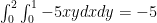 which is far more believable.
 and the planes
  ; the plane
  is outside of this cylinder. (


 find
find  That is fairly straight forward, no? But there is a bit more here than meets the eye, as I quickly found out. I graphed this on Desmos and:
 which leads to families of lines with either slope 1 or slope negative 1 and y intercepts multiples of
 which leads to:
 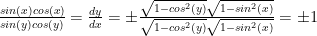 by both the original equation and the circle identity.
 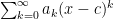 , the most important thing is to determine the open interval of absolute convergence; that is, the intervals on which
  converges.
  (that is, at
  only, on some open interval
  or the whole real line. Side note: this is an interesting place to point out the influence that the calculus of complex variables has on real variable calculus! These open intervals are the most important aspect as one can prove that one can differentiate and integrate said series “term by term” on the open interval of absolute convergence; sometimes
  .
. ; here we see that for
  ,
,  and is equal to
  for
for  ; to show this do the old “shifted sum” addition:
  ,
,  then subtract:
  as most of the terms cancel with the subtraction.
  the “n’th partial sum, then the series
  converges if an only if the sequence of partial sums
  converges; yes there are
  and we get convergence if
  goes to zero, which happens only if
  .
.  has all
  (suppressing the indices).
 , then if
  is the sequence in question, there has to be some
  such that
  for any small, positive
  . Then because
  for all
 converges (standard convergence) then
  as a sequence. This is pretty clear if the
  are non-negative; the idea is that the sequence of partial sums
  becomes arbitrarily small. Of course, this is true even if the terms are not all positive.
 and
and  converges, then so does
  . If
. If  converges. Now, of course, absolute convergence implies convergence:
 and if
  converges by direct comparison. Now note
  is the difference of two convergent series:
  and therefore converges.
  is a non-negative, non-decreasing function on some
  (that is,
  ) Then
  converges if and only if
  converges as an improper integral.
 is just a right endpoint Riemann sum for
  is the right endpoint estimate for
 certainly has
  diverging.
![f(x) = \begin{cases} 2^n , & \text{ if } x \in [n, n+2^{-2n}] \\0, & \text{ otherwise} \end{cases}](https://s0.wp.com/latex.php?latex=f%28x%29+%3D+%5Cbegin%7Bcases%7D++2%5En+%2C+%26+%5Ctext%7B+if+%7D++x+%5Cin+%5Bn%2C+n%2B2%5E%7B-2n%7D%5D+%5C%5C0%2C+%26+%5Ctext%7B+otherwise%7D+%5Cend%7Bcases%7D+&bg=ffffff&fg=000000&s=0&c=20201002) gives an unbounded function with unbounded sum
gives an unbounded function with unbounded sum  but the integral converges to the sum
  . The “boxes” get taller and skinnier.
 converges if
  and diverges otherwise. Proof: Integral test.
 and
and 
 then so does
  then so does
  then
then  such that
  This means
  and we get convergence by direct comparison. See how useful that test is?
 to exist; for the convergence case it is only necessary that there be some
  for which
  ; if one is familiar with the
 clearly converges, but nailing down the proof with direct comparison can be hard. But a limit comparison with
  is pretty easy.
 (if the limit exists..if it doesn’t..stay tuned).
 the series converges. If
  the series diverges. If
  the test is inconclusive.
  such that for all
  we have
  then the series converges (we can use the
 to obtain
 See where this is going: each ratio is less than
  so we have:
 which is a convergent geometric series.
  we have
  then the series converges (exercise: find the “divergence version”).
  so the original series converges by direction comparison.
 and therefore converges by direct comparison. And the limsup version of the root test works as well.
  which is unbounded..but
  .
.  converges but does NOT converge absolutely (p-test). On one hand, such series are a LOT of fun..but the convergence is very slow and unstable and so might say that these series are not as important as the series that converges absolutely. But there is a lot of interesting mathematics to be had here.
 and for all
  .
. converges if and only if
  (as the magnitudes get steadily smaller) and below by
  (same reason. Note also that
  so the sequence of partial sums of even index are an increasing bounded sequence and therefore converges to some limit, say,
  . But
. But  and so by a routine “epsilon-N” argument the odd partial sums converge to
  as well.
  . Note: this could be 0 terms. Now use the negative terms to go of the left of
  Then move to the right, past
  . Then go back again to get
  to the left of
  and the
  bracket
  .
. and you are told to calculate the derivative?

 to obtain

 ? The derivative certainly exists there but what about that second factor? Yes, the sin(x) gets cancelled out by the first factor, but AS WRITTEN, there is an oh-so-subtle problem with domains.
  only after simplifying ..which one might see as a limit process.
 and then took the log of both sides. Where is the log defined? And when does
  ? You got it: this only works when
  .
. is justified only when each
  .
. is a differentiable function then
 material but here goes: write
 we get
  as usual. If
  then
then  and so in either case:
 where
where  : just calculate
  . noting that
 ?
? is a product of differentiable functions and
 then
then
 are differentiable and
  . Then
  and
and 
 . Then
  and
and 
 then
then  by inductive application of 1.
 then let
  as in 2. Then by 2, we have
  Now this quantity is zero unless
  and
and  . But in this case note that
 is
is  at integer points over an interval of width
  and was zero elsewhere.
  was such a series.
  converges (either conditionally or absolutely) for some
  then the series converges absolutely for all
  where
where  The proof isn’t hard; note that convergence of
  for some positive
  and then
  and compare to a convergent geometric series. Mind you, he was teaching series at the time..and yes, is a senior, research active faculty member with years and years of experience; he mentored me so many years ago.
 if
if  is rational,
  if
if  (try:
(try:  at
at 