infinite series | College Math Teaching

May 25, 2021

Power series: review for inexperienced calculus teachers

This is “part 2” of a previous post about series. Once again, this is not designed for students seeing the material for the first time.

I’ll deal with general power series first, then later discuss Taylor Series (one method of obtaining a power series).

General Power Series Unless otherwise stated, we will be dealing with series such as $\sum a_n x^n$ though, of course, a series can expanded about any point in the real line (e. g. $\sum a_n (x-c)^n$ ) Note: unless it is needed, I’ll be suppressing the index in the summation sign.

So, IF we have a function $f(x) = \sum a_n x^n = a_0 + a_1 x + a_2 x^2 + ....a_k x^k + a_{k+1} x^{k+1}$ ..

what do we mean by this and what can we say about it?

The first thing to consider, of course, is convergence. One main fact is that the open interval of convergence of a power series centered at 0 is either:
1. Non existent …series converges at $x = 0$ only (e. g. $\sum_{k=0} (k!)x^k$ ; try the ratio test) or

2. Converges absolutely on $(-r, r)$ for some $r >0$ and diverges for all $|x| > r$ (like a geometric series) (anything possible for $|x| = r$ ) or

3. Converges absolutely on the whole real line.

Many texts state this result but do not prove it. I can understand as this result is really an artifact of calculus of a complex variable. But it won’t hurt to sketch out a proof at least for the “converge” case for $(-r, r)$ so I’ll do that.

So, let’s assume that $\sum a_n c^n$ converges (either absolute OR conditional ) So, by the divergence test, we know that the sequence of terms $a_n c^n \rightarrow 0$ . So we can find some index $M$ such that $n > M \rightarrow |a_n c^n| < 1$

So write: $|a_n x^n| = |a_n||c^n||| {x^n \over c^n} | < | {x^n \over c^n} |$ and $\sum | {x^n \over c^n} |$ converges absolutely for $|x| < |c|$ . The divergence follows from a simple “reversal of the inequalities (that is, if the series diverged at $x = c$ ).

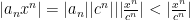
Though the relation between real and complex variables might not be apparent, it CAN be useful. Here is an example: suppose one wants to find the open interval of convergence of, say, the series representation for ${1 \over 3+2x^2 }$ ? Of course, the function itself is continuous on the whole real line. But to find the open interval of convergence, look for the complex root of $3+2 x^2$ that is closest to zero. That would be $x = \sqrt{{3 \over 2}} i$ so the interval is $|x| < \sqrt{{3 \over 2}}$

So, what about a function defined as a power series?

For one, a power series expansion of a function at a specific point (say, $x =0$ ) is unique:

Say $a_0 + a_1 x + a_2 x^2 + a_3 x^3..... = b_0 + b_1 x + b_2 x^2 + b_3 x^3 ....$ on the interval of convergence, then substituting $x=0$ yields $a_0 = b_0$ . So subtract from both sides and get: $a_1 x + a_2 x^2 + a_3 x^3.. = b_1 x + b_2 x^2 + b_3 x^3 ...$ . Now assuming one can “factor out an x” from both sides (and you can) we get $a_1 = b_1$ , etc.

Yes, this should have property been phrased as a limit and I’ve yet to show that $f(x) = \sum a_n x^n$ is continuous on its open interval of absolute convergence.

Now if you say “doesn’t that follow from uniform convergence which follows from the Weierstrass M test” you’d be correct…and you are probably wasting your time reading this.

Now if you remember hearing those words but could use a refresher, here goes:

We want $|f(x) -f(t)| < \epsilon$ for $x, t$ sufficiently close AND both within the open interval of absolute convergence, say $(-r, r)$ Choose $s < r$ where $|s| > max(|x|, |t|)$ and $M$ such that ${\epsilon \over 4} > \sum_{k=M} |a_k s^k|$ and $\delta >0$ where $|x-t| < \delta \rightarrow {\epsilon \over 2 } >| \sum_{k=0} ^{M-1} a_k x^k - \sum_{k=0} ^{M-1} a_k t^k |$ (these are just polynomials).

The rest follows: $|f(x) -f(t)| = | \sum_{k=0} ^{M-1} a_k x^k - \sum_{k=0} ^{M-1} a_k t^k + \sum_{k=M} |a_k x^k| - \sum_{k=M} |a_k t^k| | \leq | \sum_{k=0} ^{M-1} a_k x^k - \sum_{k=0} ^{M-1} a_k t^k | + 2 | \sum_{k=M} |a_k s^k| | \leq \epsilon$

Calculus On the open interval of absolute convergence, a power series can be integrated term by term and differentiated term by term. Neither result, IMHO, is “obvious.” In fact, sans extra criteria, for series of functions, in general, it is false. Quickly: if you remember Fourier Series, think about the Fourier series for a rectangular pulse wave; note that the derivative is zero everywhere except for the jump points (where it is undefined), then differentiate the constituent functions and get a colossal mess.

Differentiation: most texts avoid the direct proof (with good reason; it is a mess) but it can follow from analysis results IF one first shows that the absolute (and uniform) convergence of $\sum a_n x^n$ implies the absolute (and uniform) convergence of $\sum n a_n x^{n-1}$

So, let’s start here: if $\sum a_n x^n$ is absolutely convergent on $(-r, r)$ then so is $\sum a_n nx^{n-1}$ .

Here is why: because we are on the open interval of absolute convergence, WLOG, assume $x > 0$ and find $s > 0$ where $\sum a_n (x+s)^n$ is also absolutely convergent. Now, note that $(x+s)^n = x^n + s nx^{n-1} + ...s^n > snx^{n-1}$ so the series $s \sum a_n nx^{n-1}$ converges by direct comparison on $(-r, r)$ which establishes what we wanted to show.

Of course, this doesn’t prove that the expected series IS the derivative; we have a bit more work to do.

Again, working on the open interval of absolute convergence, let’s look at:

$lim_{x \rightarrow t} {f(x) -f(t) \over x-t } = lim_{x \rightarrow t} {1 \over x-t} (\sum a_n x^n -\sum a_n t^n)$

Now, we use the fact that $\sum a_n n x^{n-1}$ is absolutely convergent on $(-r, r)$ and given any $\epsilon > 0$ we can find $M > 0$ so that $n > m \rightarrow \sum_{n} a_k k s^{k-1}$ for $s$ between $x$ and $t$

So let’s do that: pick $\epsilon >0$ and then note:

$lim_{x \rightarrow t} {1 \over x-t} (\sum a_n x^n -\sum a_n t^n) =$

$lim_{x \rightarrow t} {1 \over x-t} (\sum_{k=0}^{n-1}a_k( x^k-t^k) ) +\sum_{k=n} a_k (x^k-t^n) ) =$

$lim_{x \rightarrow t} \sum_{k=0}^{n-1} a_k {x^k-t^k \over x-t} + \sum_{k=n} a_k {x^k-t^n \over x-t}$

$= \sum_{k=1}^{n-1} a_k k x^{k-1} + lim_{x \rightarrow t} \sum_{k=n} a_k {x^k-t^n \over x-t}$

Now apply the Mean Value Theorem to each term in the second term:

$= \sum_{k=1}^{n-1} a_k k x^{k-1} + lim_{x \rightarrow t} \sum_{k=n} a_k k(s_k)^{k-1}$ where each $s_k$ is between $x$ and $t$ . By the choice of $n$ the second term is less than $\epsilon$ , which is arbitrary, and the first term is the first $n$ terms of the “expected” derivative series.

So, THAT is “term by term” differentiation…and notice that we’ve used our hypothesis …almost all of it.

Term by term integration

Theoretically, integration combines easier with infinite summation than differentiation does. But given we’ve done differentiation, we can then do anti-differentiation by showing that $\sum a_k {x^{k+1} \over k+1}$ converges and then differentiating.

But let’s do this independently; it is good for us. And we’ll focus on the definite integral.

$\int^b_a \sum a_k x^k dx =$ (of course, $[a,b] \subset (-r, r)$ )

Once again, choose $n$ so that $\sum_{k=n} a_k x^k < \epsilon$

Then $\int^b_a \sum a_k x^k dx = \int^b_a \sum_{k=0}^{n-1} a_kx^k dx + \int^b_a \sum_{k=n} a_k x^k dx$ and this is less than (or equal to)

$\sum_{k=0}^{n-1} \int^b_a a_kx^k dx + \epsilon (b-a)$

But $\epsilon$ is arbitrary and so the result follows, for definite integrals. It is an easy exercise in the Fundamental Theorem of Calculus to extract term by term anti-differentiation.

Taylor Series

Ok, now that we can say stuff about a function presented as a power series, what about finding a power series representation for a function, PROVIDED there is one? Note: we’ll need the function to have an infinite number of derivatives on an open interval about the point of expansion. We’ll also need another condition, which we will explain as we go along.

We will work with expanding about $x = 0$ . Let $f(x)$ be the function of interest and assume all of the relevant derivatives exist.

Start with $\int^x_0 f'(t) dt = f(x) -f(0) \rightarrow f(x) =f(0) + \int ^x_0 f'(t) dt$ which can be thought of as our “degree 0” expansion plus remainder term.

But now, let’s use integration by parts on the integral with $u = f'(t), dv = dt, du = f''(t) and v = (t-x)$ (it is a clever choice for $v$ ; it just has to work.

So now we have: $f(x) = f(0) + |^x_0 f'(t)(t-x) - \int^x_0f''(t) (t-x) dt = f(0) + xf'(0) - \int^x_0f''(t) (t-x) dt$

It looks like we might run into sign trouble on the next iteration, but we won’t as we will see: do integration by parts again:

$u =f''(t), dv = (t-x), du = f'''(t), v = {1 \over 2} (t-x)^2$ and so we have:

$f(x) =f(0) + xf'(0) -( |^x_0 f''(t) {1 \over 2}(t-x)^2 -{1 \over 2} \int^x_0 f'''(t)(t-x)^2 dt$

This turns out to be $f(0) +xf'(0) +{1 \over 2} f''(0)x^2 + \int^x_0 f'''(t) (t-x)^2 dt$ .

An induction argument yields

$f(x) = \sum^n_{k=0} f^{(k)}{1 \over k!}x^k +{1 \over n} \int^x_0 f^{(n+1)}(t) (t-x)^n dt$

For the series to exist (and be valid over an open interval) all of the derivatives have to exist and;

$lim_{n \rightarrow \infty} {1 \over n!} \int^x_0 f^{(n+1)}(t) (t-x)^n dt = 0$ .

Note: to get the Lagrange remainder formula that you see in some texts, let $M = max \{|f^{(n+1)} (t) \}$ for $t \in [0,x]$ and then $| {1 \over n!} \int^x_0 f^{(n+1)}(t) (t-x)^n dt | \leq {1 \over n!} M \int^x_0 (t-x)^n dt| = {M \over (n+1)!}| |^x_0(t-x)^{(n+1)} | =M{x^{(n+1)} \over (n+1)!}$

It is a bit trickier to get the equality $f^{(n+1)}(\eta) {x^{n+1} \over (n+1)!}$ as the error formula; it is a Mean Value Theorem for integrals calculation.

About the remainder term going to zero: this is necessary. Consider the classic counterexample:

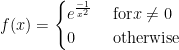
$f(x) = \begin{cases} e^{-1 \over x^2} & \text{ for} x \neq 0 \\ 0 & \text{ otherwise} \end{cases}$

It is an exercise in the limit definition and L’Hopital’s Rule to show that $f^{(k)} (0) = 0$ for all $k \in \{0, 1, 2, ... \}$ and so a Taylor expansion at zero is just the zero function, and this is valid at 0 only.

As you can see, the function appears to flatten out near x =0 $ but it really is NOT constant.

Note: of course, using the Taylor method isn’t always the best way. For example, if we were to try to get the Taylor expansion of ${1 \over 1+x^2}$ at $x = 0$ it is easier to use the geometric series for ${1 \over 1-u}$ and substitute $u= -x^2$ ; the uniqueness of the power series expansion allows for that.

May 10, 2021

Series convergence tests: the “harder to use in calculus 1” tests may well be the most useful.

Filed under: algebra, calculus, infinite series, linear albegra, matrix algebra, sequences, series, Taylor Series — oldgote @ 3:17 pm

I talked about the root and ratio test here and how the root test is the stronger of the two tests. What I should point out that the proof of the root test depends on the basic comparison test.

And so..a professor on Twitter asked:

https://twitter.com/MathProfPeter/status/1385606921156284429

Of course, one proves the limit comparison test by the direct comparison test. But in a calculus course, the limit comparison test might appear to be more readily useful..example:

Show $\sum {1 \over k^2-1}$ converges.

So..what about the direct comparison test?

As someone pointed out: the direct comparison can work very well when you don’t know much about the matrix.

One example can be found when one shows that the matrix exponential $e^A$ where $A$ is a $n \times n$ matrix.

For those unfamiliar: $e^A = \sum^{\infty}_{k=0} {A^k \over k!}$ where the powers make sense as $A$ is square and we merely add the corresponding matrix entries.

What enables convergence is the factorial in the denominators of the individual terms; the i-j’th element of each $A^k$ can get only so large.

But how does one prove convergence?

The usual way is to dive into matrix norms; one that works well is $|A| = \sum_{(i,j)} |a_{i,j}|$ (just sum up the absolute value of the elements (the Taxi cab norm or $l_1$ norm )

Then one can show $|AB| \leq |A||B|$ and $|a_{i,j}| \leq |A|$ and together this implies the following:

For any index $k$ where $a^k_{i,j}$ is the i-j’th element of $A^k$ we have:

$| a^k_{i,j} | \leq |A^k| \leq |A|^k$

It then follows that $| [ e^A ]_{i,j} | \leq \sum^{\infty}_{k=0} {|A^k |\over k!} \leq \sum^{\infty}_{k=0} {|A|^k \over k!} =e^{|A|}$ . Therefore every series that determines an entry of the matrix $e^A$ is an absolutely convergent series by direct comparison. and is therefore a convergent series.

Comments (1)

February 5, 2016

More fun with selective sums of divergent series

Filed under: advanced mathematics, calculus, induction, infinite series, number theory, sequences — Tags: divergent series, harmonic series, select sum of a series — collegemathteaching @ 1:56 am

Just a reminder: if $\sum_{k=1}^{\infty} a_k$ is a series and $c_1, c_2, ...c_n ,,$ is some sequence consisting of 0’s and 1’s then a selective sum of the series is $\sum_{k=1}^{\infty} c_k a_k$ . The selective sum concept is discussed in the MAA book Real Infinite Series (MAA Textbooks) by Bonar and Khoury (2006) and I was introduced to the concept by Ferdinands’s article Selective Sums of an Infinite Series in the June 2015 edition of Mathematics Magazine (Vol. 88, 179-185).

There is much of interest there, especially if one considers convergent series or alternating series.

This post will be about divergent series of positive terms for which $lim_{n \rightarrow \infty} a_n = 0$ and $a_{n+1} < a_n$ for all $n$ .

The first fun result is this one: any selected $x > 0$ is a selective sum of such a series. The proof of this isn’t that bad. Since $lim_{n \rightarrow \infty} a_n = 0$ we can find a smallest $n$ such that $a_n \leq x$ . Clearly if $a_n = x$ we are done: our selective sum has $c_n = 1$ and the rest of the $c_k = 0$ .

If not, set $n_1 = n$ and note that because the series diverges, there is a largest $m_1$ so that $\sum_{k=n_1}^{m_1} a_k \leq x$ . Now if $\sum_{k=n_1}^{m_1} a_k = x$ we are done, else let $\epsilon_1 = x - \sum_{k=n_1}^{m_1} a_k$ and note $\epsilon_1 < a_{m_1+1}$ . Now because the $a_k$ tend to zero, there is some first $n_2$ so that $a_{n_2} \leq \epsilon_1$ . If this is equality then the required sum is $a_{n_2} + \sum_{k=n_1}^{m_1} a_k$ , else we can find the largest $m_2$ so that $\sum_{k=n_1}^{m_1} a_k + \sum_{k=n_2}^{m_2} a_k \leq x$

This procedure can be continued indefinitely. So if we label $\sum_{k=n_j}^{m_{j}} a_k = s_j$ we see that $s_1 + s_2 + ...s_{n} = t_{n}$ form an increasing, bounded sequence which converges to the least upper bound of its range, and it isn’t hard to see that the least upper bound is $x$ because $x-t_{n} =\epsilon_n < a_{m_n+1}$

So now that we can obtain any positive real number as the selective sum of such a series, what can we say about the set of all selective sums for which almost all of the $c_k = 0$ (that is, all but a finite number of the $c_k$ are zero).

Answer: the set of all such selective sums are dense in the real line, and this isn’t that hard to see, given our above construction. Let $(a,b)$ be any open interval in the real line and let $a < x < b$ . Then one can find some $N$ such that for all $n > N$ we have $x - a_n > a$ . Now consider our construction and choose $m$ large enough such that $x - t_m > x - a_n > a$ . Then the $t_m$ represents the finite selected sum that lies in the interval $(a,b)$ .

We can be even more specific if we now look at a specific series, such as the harmonic series $\sum_{k=1}^{\infty} \frac{1}{k}$ . We know that the set of finite selected sums forms a dense subset of the real line. But it turns out that the set of select sums is the rationals. I’ll give a slightly different proof than one finds in Bonar and Khoury.

First we prove that every rational in $(0,1]$ is a finite select sum. Clearly 1 is a finite select sum. Otherwise: Given $\frac{p}{q}$ we can find the minimum $n$ so that $\frac{1}{n} \leq \frac{p}{q} < \frac{1}{n-1}$ . If $\frac{p}{q} = \frac{1}{n}$ we are done. Otherwise: the strict inequality shows that $pn-p < q$ which means $pn-q < p$ . Then note $\frac{p}{q} - \frac{1}{n} = \frac{pn-q}{qn}$ and this fraction has a strictly smaller numerator than $p$ . So we can repeat our process with this new rational number. And this process must eventually terminate because the numerators generated from this process form a strictly decreasing sequence of positive integers. The process can only terminate when the new faction has a numerator of 1. Hence the original fraction is some sum of fractions with numerator 1.

Now if the rational number $r$ in question is greater than one, one finds $n_1$ so that $\sum^{n_1}_{k=1} \frac{1}{k} \leq r$ but $\sum^{n_1+1}_{k=1} \frac{1}{k} > r$ . Then write $r-\sum^{n_1+1}_{k=1} \frac{1}{k}$ and note that its magnitude is less than $\frac{1}{n_1+1}$ . We then use the procedure for numbers in $(0,1)$ noting that our starting point excludes the previously used terms of the harmonic series.

There is more we can do, but I’ll stop here for now.

April 6, 2013

Calculus and Analysis: the power of examples

Filed under: advanced mathematics, analysis, calculus, infinite series, integrals, Lebesgue Integration — Tags: absolutely continuous, analysis, bounded variation, squeeze theorem — collegemathteaching @ 7:06 pm

In my non-math life I am an avid runner and walker. Ok, my enthusiasm for these sports greatly excedes my talent and accomplishments for these sports; I once (ONCE) broke 40 minutes for the 10K run and that was in 1982; the winner (a fellow named Bill Rodgers) won that race and finished 11 minutes ahead of me that day! 🙂 Now I’ve gotten even slower; my fastest 10K is around 53 minutes and I haven’t broken 50 since 2005. 😦

But alas I got a minor bug and had to skip today’s planned races; hence I am using this morning to blog about some math.

Real Analysis and Calculus
I’ve said this before and I’ll say it again: one of my biggest struggles with real analysis and calculus was that I often didn’t see the point of the nuances in the proof of the big theorems. My immature intuition was one in which differentiable functions were, well, analytic (though I didn’t know that was my underlying assumption at the time). Their graphs were nice smooth lines, though I knew about corners (say, $f(x) = |x|$ at $x = 0$ .

So, it appears to me that one of the way we can introduce the big theorems (along with the nuances) is to have a list of counter examples at the ready and be ready to present these PRIOR to the proof; that way we can say “ok, HERE is why we need to include this hypothesis” or “here is why this simple minded construction won’t work.”

So, what are my favorite examples? Well, one is the function $f(x) =\left\{ \begin{array}{c}e^{\frac{-1}{x^2}}, x \ne 0 \\ 0, x = 0 \end{array}\right.$ is a winner. This gives an example of a $C^{\infty}$ function that is not analytic (on any open interval containing 0 ).

The family of examples I’d like to focus on today is $f(x) =\left\{ \begin{array}{c}x^ksin(\frac{\pi}{ x}), x \ne 0 \\ 0, x = 0 \end{array}\right.$ , $k$ fixed, $k \in {1, 2, 3,...}$ .

Note: henceforth, when I write $f(x) = x^ksin(\frac{\pi}{x})$ I’ll let it be understood that I mean the conditional function that I wrote above.

Use of this example:
1. Squeeze theorem in calculus: of course, $|x| \ge |xsin(\frac{\pi}{x})| \ge 0$ ; this is one time we can calculate a limit without using a function which one can merely “plug in”. It is easy to see that $lim_{x \rightarrow 0 } |xsin(\frac{\pi}{x})| = 0$ .

2. Use of the limit definition of derivative: one can see that $lim_{h \rightarrow 0 }\frac{h^2sin(\frac{\pi}{h}) - 0}{h} =0$ ; this is one case where we can’t merely “calculate”.

3. $x^2sin(\frac{\pi}{x})$ provides an example of a function that is differentiable at the origin but is not continuously differentiable there. It isn’t hard to see why; away from 0 the derivative is $2x sin(\frac{\pi}{x}) - \pi cos(\frac{\pi}{x})$ and the limit as $x$ approaches zero exists for the first term but not the second. Of course, by upping the power of $k$ one can find a function that is $k-1$ times differentiable at the origin but not $k-1$ continuously differentiable.

4. The proof of the chain rule. Suppose $f$ is differentiable at $g(a)$ and $g$ is differentiable at $a$ . Then we know that $f(g(x))$ is differentiable at $x=a$ and the derivative is $f'(g(a))g'(a)$ . The “natural” proof (say, for $g$ non-constant near $x = a$ looks at the difference quotient: $lim_{x \rightarrow a} \frac{f(g(x))-f(g(a))}{x-a} =lim_{x \rightarrow a} \frac{f(g(x))-f(g(a))}{g(x)-g(a)} \frac{g(x)-g(a)}{x-a}$ which works fine, so long as $g(x) \ne g(a)$ . So what could possibly go wrong; surely the set of values of $x$ for which $g(x) = g(a)$ for a differentiable function is finite right? 🙂 That is where $x^2sin(\frac{\pi}{x})$ comes into play; this equals zero at an infinite number of points in any neighborhood of the origin.

Hence the proof of the chain rule needs a workaround of some sort. This is a decent article on this topic; it discusses the usual workaround: define $G(x) =\left\{ \begin{array}{c}\frac{f(g(x))-f(g(a))}{g(x)-g(a)}, g(x)-g(a) \ne 0 \\ f'(g(x)), g(x)-g(a) = 0 \end{array}\right.$ . Then it is easy to see that $lim_{x \rightarrow a} \frac{f(g(x))-f(g(a))}{x-a} = lim_{x \rightarrow a}G(x)\frac{g(x)-g(a)}{x-a}$ since the second factor of the last term is zero when $x = a$ and the limit of $G(x)$ exists at $x = a$ .

Of course, one doesn’t have to worry about any of this if one introduces the “grown up” definition of derivative from the get-go (as in: best linear approximation) and if one has a very gifted class, why not?

5. The concept of “bounded variation” and the Riemann-Stiltjes integral: given functions $f, g$ over some closed interval $[a,b]$ and partitions $P$ look at upper and lower sums of $\sum_{x_i \in P} f(x_i)(g(x_{i}) - g(x_{i-1}) = \sum_{x_i \in P}f(x_i)\Delta g_i$ and if the upper and lower sums converge as the width of the partions go to zero, you have the integral $\int^b_a f dg$ . But this works only if $g$ has what is known as “bounded variation”: that is, there exists some number $M > 0$ such that $M > \sum_{x_i \in P} |g(x_i)-g(x_{i-1})|$ for ALL partitions $P$ . Now if $g(x)$ is differentiable with a bounded derivative on $[a,b]$ (e. g. $g$ is continuously differentiable on $[a,b]$ then it isn’t hard to see that $g$ had bounded variation. Just let $W$ be a bound for $|g'(x)|$ and then use the Mean Value Theorem to replace each $|g(x_i) - g(x_{i-1})|$ by $|g'(x_i^*)||x_i - x_{i-1}|$ and the result follows easily.

So, what sort of function is continuous but NOT of bounded variation? Yep, you guessed it! Now to make the bookkeeping easier we’ll use its sibling function: $xcos(\frac{\pi}{x})$ . 🙂 Now consider a partition of the following variety: $P = \{0, \frac{1}{n}, \frac{1}{n-1}, ....\frac{1}{3}, \frac{1}{2}, 1\}$ . Example: say $\{0, \frac{1}{5}, \frac{1}{4}, \frac{1}{3}, \frac{1}{2}, 1\}$ . Compute the variation: $|0-(- \frac{1}{5})|+ |(- \frac{1}{5}) - \frac{1}{4}| + |\frac{1}{4} - (-\frac{1}{3})|+ |-\frac{1}{3} - \frac{1}{2}| + |\frac{1}{2} -(-1)| = \frac{1}{5} + 2(\frac{1}{4} + \frac{1}{3} + \frac{1}{2}) + 1$ . This leads to trouble as this sum has no limit as we progress with more points in the sequence of partitions; we end up with a divergent series (the Harmonic Series) as one term as points are added to the partition.

6. The concept of Absolute Continuity: this is important when one develops the Fundamental Theorem of Calculus for the Lebesgue integral. You know what it means for $f$ to be continuous on an interval. You know what it means for $f$ to be uniformly continuous on an interval (basically, for the whole interval, the same $\delta$ works for a given $\epsilon$ no matter where you are, and if the interval is a closed one, an easy “compactness” argument shows that continuity and uniform continuity are equivalent. Absolute continuity is like uniform continuity on steroids. I’ll state it for a closed interval: $f$ is absolutely continuous on an interval $[a,b]$ if, given any $\epsilon > 0$ there is a $\delta > 0$ such that for $\sum |x_{i}-y_{i}| < \delta, \sum |f(x_i) - f(y_{i})| < \epsilon$ where $(x_i, y_{i})$ are pairwise disjoint intervals. An example of a function that is continuous on a closed interval but not absolutely continuous? Yes; $f(x) = xcos(\frac{\pi}{x})$ on any interval containing $0$ is an example; the work that we did in paragraph 5 works nicely; just make the intervals pairwise disjoint.

July 15, 2011

Quantum Mechanics and Undergraduate Mathematics III: an example of a state function

Filed under: advanced mathematics, analysis, applied mathematics, calculus, Fourier Series, infinite series, linear albegra, physics, quantum mechanics, science — collegemathteaching @ 1:59 am

I feel bad that I haven’t given a demonstrative example, so I’ll “cheat” a bit and give one:

For the purposes of this example, we’ll set our Hilbert space to the the square integrable piecewise smooth functions on $[-\pi, \pi]$ and let our “state vector” $\psi(x) =\left\{ \begin{array}{c}1/\sqrt{\pi}, 0 < x \leq \pi \\ 0,-\pi \leq x \leq 0 \end{array}\right.$

Now consider a (bogus) state operator $d^2/dx^2$ which has an eigenbasis $(1/\sqrt{\pi})cos(kx), (1/\sqrt{\pi})sin(kx), k \in {, 1, 2, 3,...}$ and $1/\sqrt{2\pi}$ with eigenvalues $0, -1, -4, -9,......$ (note: I know that this is a degenerate case in which some eigenvalues share two eigenfunctions).

Note also that the eigenfunctions are almost the functions used in the usual Fourier expansion; the difference is that I have scaled the functions so that $\int^{\pi}_{-\pi} (sin(kx)/\sqrt{\pi})^2 dx = 1$ as required for an orthonormal basis with this inner product.

Now we can write $\psi = 1/(2 \sqrt{\pi}) + 4/(\pi^{3/2})(sin(x) + (1/3)sin(3x) + (1/5)sin(5x) +..)$
(yes, I am abusing the equal sign here)
This means that $b_0 = 1/\sqrt{2}, b_k = 2/(k \pi), k \in {1,3,5,7...}$

Now the only possible measurements of the operator are 0, -1, -4, -9, …. and the probability density function is: $p(A = 0) = 1/2, P(A = -1) = 4/(\pi^2), P(A = -3) = 4/(9 \pi^2),...P(A = -(2k-1))= 4/(((2k-1)\pi)^2)..$

One can check that $1/2 + (4/(\pi^2))(1 + 1/9 + 1/25 + 1/49 + 1/81....) = 1.$

Here is a plot of the state function (blue line at the top) along with some of the eigenfunctions multiplied by their respective $b_k$ .

Comments (3)

April 3, 2011

Infinite Series: the Root and Ratio tests

Filed under: advanced mathematics, analysis, calculus, infinite series, series — collegemathteaching @ 3:29 am

This post is written mostly for those who are new to teaching calculus rather than for students learning calculus for the first time. Experienced calculus teachers and those whose analysis background is still fresh will likely be bored. 🙂

The setting will be series $\Sigma^\infty_{k=1} a_k$ with $a_k > 0$ We will use the usual notion of convergence; that is, the series converges if the sequence of partial sums converge. If that last statement puzzles you, there are other non-standard notions of convergence.

I’ll give the usual statements of the root test and the ratio test, given $\Sigma^\infty_{k=1} a_k$ with $a_k > 0$

Root Test
Suppose $lim_{k \rightarrow \infty}(a_k)^{\frac{1}{k}} = c$ . If $c >1$ the series diverges. If $c < 1$ the series converges. If $c = 1$ the test is inconclusive.

Ratio Test
Suppose $lim_{k \rightarrow \infty} a_{k+1}/a_k = c$ . If $c >1$ the series diverges. If $c < 1$ the series converges. If $c = 1$ the test is inconclusive.

Quick examples of how these tests are used
Example one: show that $\Sigma^{\infty}_{k=1} (x/k)^{k}$ converges for all $x$ . Apply the root test and note $lim_{k \rightarrow \infty} ((x/k))^{k})^{1/k} = lim_{k \rightarrow \infty} ((x/k) = 0$ for all $x \geq 0$ hence the series converges absolutely for all $x$ .

Example two: show that show that $\Sigma^{\infty}_{k=1} (x^k/k!)$ converges for all $x$ . Consider $lim_{k \rightarrow \infty} (x^{k+1}/(k+1)!)/((x^k)/k!) = lim_{k \rightarrow \infty} x/(k+1) = 0 < 1$ for all $x \geq 0$ hence the series converges absolutely for all $x$ .

However these tests, as taught, are often more limited than they need to be. For example, if one considers the series $\Sigma^{\infty}_{k=1} (|sin(k)|/2)^{k}$ the root test, as stated, doesn't apply as $lim_{k \rightarrow \infty} ((|sin(k)|)/2)^{k})^{1/k}$ fails to exist, though it is clear that the $sup{((|sin(k)|)/2)^{k})^{1/k}} = 1/2$ and the series is dominated by the convergent geometric series $\Sigma^{\infty}_{k=1} (1/2)^k$ and therefore converges.

There is also a common misconception that the root test and the ratio tests are equivalent. They aren’t; in fact, we’ll show that if a series passes the ratio test, it will also pass the root test but that the reverse is false. We’ll also provide an easy to understand stronger version of these two tests. The stronger versions should be easily within the grasp of the best calculus students and within the grasp of beginning analysis/advanced calculus students.

Note: there is nothing original here; I can recommend the books Counterexamples in Analysis by Bernard R. Gelbaum and Theory and Application of Infinite Series by Konrad Knop for calculus instructors who aren’t analysts. Much of what I say can be found there in one form or another.

The proofs of the tests and what can be learned
Basically, both proofs are merely basic comparisons with a convergent geometric series.

Proof of the root test (convergence)
If $lim_{k \rightarrow \infty} (a_k)^{1/k} = c$ with $c < 1$ then there exists some $d <1$ and some index $N$ such that for all $n > N$ , ${a_n}^{1/n} < d$ . Hence for all $n> N$ , ${a_n} < d^n$ where $d < 1$ . Therefore the series converges by a direct comparison with the convergent geometric series $\Sigma^{\infty}_{k = N} d^{k}$ .

Note the following: requiring $lim_{k \rightarrow \infty} (a_k)^{1/k}$ to exist is overkill; what is important that, for some index $N$ , $k$ , $sup_{k>N} (a_k)^{1/k} < c < 1$ . This is enough for the comparison with the geometric series to work. In fact, in the language of analysis, we can replace the limit condition with $limsup (a_k)^{1/k} = c < 1$ . If you are fuzzy about limit superior, this is a good reference.

In fact, we can weaken the hypothesis a bit further. Since the convergence of a series really depends on the convergence of the “tail” of a series, we really only need: for some index $N$ and all $n > N$ , $limsup (a_{N+k})^{1/k} = c < 1$ , $k \in \{0, 1, 2,...\}$ . This point may seem pedantic but we’ll use this in just a bit.

Note: we haven’t talked about divergence; one can work out a stronger test for divergence by using limit inferior.

Proof of the ratio test (convergence)
We’ll prove the stronger version of the ratio test: if $limsup a_{k+1}/a_k = c < 1$ then there is an index $N$ and some number $d < 1$ such that for all $n\geq N$ , $a_{n+1}/a_n < d$ .
Simple algebra implies that $a_{n+1} < (a_n)d$ and $a_{n+2} < (a_{n+1})d < (a_n)d^2$ and in general $a_{n+j} < (a_n)d^j$ . Hence the series $\Sigma ^{\infty}_{k = N} a_k$ is dominated by $(a_N)(\Sigma ^{\infty}_{k = 0} d^k)$ which is a convergent geometric series.

Comparing the root and the ratio tests
Consider the convergent series $1/2 + (1/3)^2 + (1/2)^3 + (1/3)^4 +.....+ (1/2)^{2k- 1} + (1/3)^{2k}....$ .
Then clearly $limsup a_{k} = 1/2$ hence the root test works. But the ratio test yields the following:
$(a_{2k+1})/a_{2k} = (1/2)^{2k+1}/(1/3)^{2k} = (3/2)^{2k}/2$ which tends to infinity as $k$ goes to infinity. Note: since the limit does not exist, the traditional ratio test doesn’t apply. The limit inferior tends to zero so a strengthened ratio test doesn’t imply divergence.

So the root test is not equivalent to the ratio test.

But suppose the ratio test yields convergence; that is:
$limsup a_{k+1}/a_k = c < 1$ . Then by the same arguments used in the proof:
$a_{N+j} < (a_N)d^j$ . Then we can take $j'th$ roots of both sides and note: $(a_{n+j})^{1/j} < d(a_n)^{1/j} < d$ hence the weakened hypothesis of the root test is met.

That is, the root test is a stronger test than the ratio test, though, of course, it is sometimes more difficult to apply.

We’ll state the tests in the stronger form for convergence; the base assumption that $\Sigma a_{k}$ has positive terms:

Root test: if there exists an index $N$ such that for all $n \leq N$ we have $limsup_{j} (a_{N+j})^{1/j} \leq c < 1$ then the series converges.

Ratio test: if $limsup (a_{k+1})/a_{k} \leq c < 1$ then the series converges.

It is a routine exercise to restate these tests in stronger form for divergence.

Comments (1)

College Math Teaching