Nate Silver’s Book: The signal and the noise: why so many predictions fail but some don’t

Reposted from my personal blog and from my Daily Kos Diary:

Quick Review
Excellent book. There are a few tiny technical errors (e. g., “non-linear” functions include exponential functions, but not all non-linear phenomena are exponential (e. g. power, root, logarithmic, etc.).
Also, experts have some (justified) quibbles with the book; you can read some of these concerning his chapter on climate change here and some on his discussion of hypothesis testing here.

But, aside from these, it is right on. Anyone who follows the news closely will benefit from it; I especially recommend it to those who closely follow science and politics and even sports.

It is well written and is designed for adults; it makes some (but reasonable) demands on the reader. The scientist, mathematician or engineer can read this at the end of the day but the less technically inclined will probably have to be wide awake while reading this.

Details
Silver sets you up by showing examples of failed predictions; perhaps the worst of the lot was the economic collapse in the United States prior to the 2008 general elections. Much of this was due to the collapse of the real estate market and falling house/property values. Real estate was badly overvalued, and financial firms made packages of investments whose soundness was based on many mortgages NOT defaulting at the same time; it was determined that the risk of that happening was astronomically small. That was wrong of course; one reason is that the risk of such an event is NOT described by the “normal” (bell shaped) distribution but rather by one that allows for failure with a higher degree of probability.

There were more things going on, of course; and many of these things were difficult to model accurately just due to complexity. Too many factors makes a model unusable; too few means that the model is worthless.

Silver also talks about models providing probabilistic outcomes: example saying that the GDP will be X in year Y is unrealistic; what we really should say that the probability of the GDP being X plus/minus “E” is Z percent.

Next Silver takes on pundits. In general: they don’t predict well; they are more about entertainment than anything else. Example: look at the outcome of the 2012 election; the nerds were right; the pundits (be they NPR or Fox News pundits) were wrong. NPR called the election “razor tight” (it wasn’t); Fox called it for the wrong guy. The data was clear and the sports books new this, but that doesn’t sell well, does it?

Now Silver looks at baseball. Of course there are a ton of statistics here; I am a bit sorry he didn’t introduce Bayesian analysis in this chapter though he may have been setting you up for it.

Topics include: what does raw data tell you about a player’s prospects? What role does a talent scout’s input have toward making the prediction? How does a baseball players hitting vary with age, and why is this hard to measure from the data?

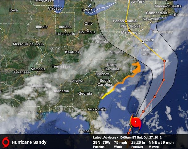
The next two chapters deal with predictions: earthquakes and weather. Bottom line: we have statistical data on weather and on earthquakes, but in terms of making “tomorrow’s prediction”, we are much, much, much further along in weather than we are on earthquakes. In terms of earthquakes, we can say stuff like “region Y has a X percent chance of an earthquake of magnitude Z within the next 35 years” but that is about it. On the other hand, we are much better about, say, making forecasts of the path of a hurricane, though these are probabilistic:

In terms of weather: we have many more measurements.

But there IS the following: weather is a chaotic system; a small change in initial conditions can mean to a large change in long term outcomes. Example: one can measure a temperature at time t, but only to a certain degree of precision. The same holds for pressure, wind vectors, etc. Small perturbations can lead to very different outcomes. Solutions aren’t stable with respect to initial conditions.

You can see this easily: try to balance a pen on its tip. Physics tells us there is a precise position at which the pen is at equilibrium, even on its tip. But that equilibrium is so unstable that a small vibration of the table or even small movement of air in the room is enough to upset it.

In fact, some gambling depends on this. For example, consider a coin toss. A coin toss is governed by Newton’s laws for classical mechanics, and in principle, if you could get precise initial conditions and environmental conditions, the outcome shouldn’t be random. But it is…for practical purposes. The same holds for rolling dice.

Now what about dispensing with models and just predicting based on data alone (not regarding physical laws and relationships)? One big problem: data is noisy and is prone to be “overfitted” by a curve (or surface) that exactly matches prior data but is of no predictive value. Think of it this way: if you have n data points in the plane, there is a polynomial of degree n-1 that will fit the data EXACTLY, but in most cases have a very “wiggly” graph that provides no predictive value.

Of course that is overfitting in the extreme. Hence, most use the science of the situation to posit the type of curve that “should” provide a rough fit and then use some mathematical procedure (e. g. “least squares”) to find the “best” curve that fits.

The book goes into many more examples: example: the flu epidemic. Here one finds the old tug between models that are too simplistic to be useful for forecasting and too complicated to be used.

There are interesting sections on poker and chess and the role of probability is discussed as well as the role of machines. The poker chapter is interesting; Silver describes his experience as a poker player. He made a lot of money when poker drew lots of rookies who had money to spend; he didn’t do as well when those “bad” players left and only the most dedicated ones remained. One saw that really bad players lost more money than the best players won (not that hard to understand). He also talked about how hard it was to tell if someone was really good or merely lucky; sometimes this wasn’t perfectly clear after a few months.

Later, Silver discusses climate change and why the vast majority of scientists see it as being real and caused (or made substantially worse) by human activity. He also talks about terrorism and enemy sneak attacks; sometimes there IS a signal out there but it isn’t detected because we don’t realize that there IS a signal to detect.

However the best part of the book (and it is all pretty good, IMHO), is his discussion of Bayes law and Bayesian versus frequentist statistics. I’ve talked about this.

I’ll demonstrate Bayesian reasoning in a couple of examples, and then talk about Bayesian versus frequentist statistical testing.

Example one: back in 1999, I went to the doctor with chest pains. The doctor, based on my symptoms and my current activity level (I still swam and ran long distances with no difficulty) said it was reflux and prescribed prescription antacids. He told me this about a possible stress test: “I could stress test you but the probability of any positive being a false positive is so high, we’d learn nothing from the test”.

Example two: suppose you are testing for a drug that is not widely used; say 5 percent of the population uses it. You have a test that is 95 percent accurate in the following sense: if the person is really using the drug, it will show positive 95 percent of the time, and if the person is NOT using the drug, it will show positive only 5 percent of the time (false positive).

So now you test 2000 people for the drug. If Bob tests positive, what is the probability that he is a drug user?

Answer: There are 100 actual drug users in this population, so you’d expect 100*.95 = 95 true positives. There are 1900 non-users and 1900*.05 = 95 false positives. So there are as many false positives as true positives! The odds that someone who tests positive is really a user is 50 percent.

Now how does this apply to “hypothesis testing”?

Consider basketball. You know that a given player took 10 free shots and made 4. You wonder: what is the probability that this player is a competent free throw shooter (given competence is defined to be, say, 70 percent).

If you just go by the numbers that you see (true: n = 10 is a pathetically small sample; in real life you’d never infer anything), well, the test would be: given the probability of making a free shot is 70 percent, what is the probability that you’d see 4 (or fewer) made free shots out of 10?

Using a calculator (binomial probability calculator), we’d say there is a 4.7 percent chance we’d see 4 or fewer free shots made if the person shooting the shots was a 70 percent shooter. That is the “frequentist” way.

But suppose you found out one of the following:
1. The shooter was me (I played one season in junior high and some pick up ball many years ago…infrequently) or
2. The shooter was an NBA player.

If 1 was true, you’d believe the result or POSSIBLY say “maybe he had a good day”.
If 2 was true, then you’d say “unless this player was chosen from one of the all time worst NBA free throw shooters, he probably just had a bad day”.

Bayesian hypothesis testing gives us a way to make and informed guess. We’d ask: what is the probability that the hypothesis is true given the data that we see (asking the reverse of what the frequentist asks). But to do this, we’d have to guess: if this person is an NBA player, what is the probability, PRIOR to this 4 for 10 shooting, that this person was 70 percent or better (NBA average is about 75 percent). For the sake of argument, assume that there is a 60 percent chance that this person came from the 70 percent or better category (one could do this by seeing the percentage of NBA players shooing 70 percent of better). Assign a “bad” percentage as 50 percent (based on the worst NBA free throw shooters): (the probability of 4 or fewer made free throws out of 10 given a 50 percent free throw shooter is .377)

Then we’d use Bayes law: (.0473*.6)/(.0473*.6 + .377*.4) = .158. So it IS possible that we are seeing a decent free throw shooter having a bad day.

This has profound implications in science. For example, if one is trying to study genes versus the propensity for a given disease, there are a LOT of genes. Say one tests 1000 genes of those who had a certain type of cancer and run a study. If we accept p = .05 (5 percent) chance of having a false positive, we are likely to have 50 false positives out of this study. So, given a positive correlation between a given allele and this disease, what is the probability that this is a false positive? That is, how many true positives are we likely to have?

This is a case in which we can use the science of the situation and perhaps limit our study to genes that have some reasonable expectation of actually causing this malady. Then if we can “preassign” a probability, we might get a better feel if a positive is a false one.

Of course, this technique might induce a “user bias” into the situation from the very start.

The good news is that, given enough data, the frequentist and the Bayesian techniques converge to “the truth”.

Summary Nate Silver’s book is well written, informative and fun to read. I can recommend it without reservation.

Just for fun: NO PROFESSORS!

This photo appeared in this College Misery post.
So, I ask you the following questions (professors are disqualified from answering):

1. What is the math on the top line “supposed” to be about?
2. What transcription error is there on the board?
3. Why are the “equals signs”, as they appear, nonsense?

Bonus question (more subtle):
if one erases the first equals sign, and move the “work” in the “vector like” object off to the side where it belongs, why is the resulting equality still (technically) incorrect?

An example to apply Bayes’ Theorem and multivariable calculus

I’ve thought a bit about the breast cancer research results and found a nice “application” exercise that might help teach students about Bayes Theorem, two-variable maximizing, critical points, differentials and the like.

I’ve been interested in the mathematics and statistics of the breast cancer screening issue mostly because it provided a real-life application of statistics and Bayes’ Theorem.

So right now, for women between 40-49, traditional mammograms are about 80 percent accurate in the sense that, if a woman who really has breast cancer gets a mammogram, the test will catch it about 80 percent of the time. The false positive rate is about 8 percent in that: if 100 women who do NOT have breast cancer get a mammogram, 8 of the mammograms will register a “positive”.
Since the breast cancer rate for women in this age group is about 1.4 percent, there will be many more false positives than true positives; in fact a woman in this age group who gets a “positive” first mammogram has about a 16 percent chance of actually having breast cancer. I talk about these issues here.

So, suppose you desire a “more accurate test” for breast cancer. The question is this: what do you mean by “more accurate”?

1. If “more accurate” means “giving the right answer more often”, then that is pretty easy to do.
Current testing is going to be wrong: if C means cancer, N means “doesn’t have cancer”, P means “positive test” and M means “negative test”, then the probability of being wrong is:
. On the other hand, if you just declared EVERYONE to be “cancer free”, you’d be wrong only 1.4 percent of the time! So clearly that does not work; the “false negative” rate is 100 percent, though the “false positive” rate is 0.

On the other hand if you just told everyone “you have it”, then you’d be wrong 98.6 percent of the time, but you’d have zero “false negatives”.

So being right more often isn’t what you want to maximize, and trying to minimize the false positives or the false negatives doesn’t work either.

2. So what about “detecting more of the cancer that is there”? Well, that is where this article comes in. Switching to digital mammograms does increase detection rate but also increases the number of false positives:

The authors note that for every 10,000 women 40 to 49 who are given digital mammograms, two more cases of cancer will be identified for every 170 additional false-positive examinations.

So, what one sees is that if a woman gets a positive reading, she now has an 11 percent of actually having breast cancer, though a few more cancers would be detected.

Is this progress?

My whole point: saying one test is “more accurate” than another test isn’t well defined, especially in a situation where one is trying to detect something that is relatively rare.
Here is one way to look at it: let the probability of breast cancer be , the probability of detection of a cancer be given by and the probability of a false positive be given by . Then the probability of a person actually having breast cancer, given a positive test is given by:
; this gives us something to optimize. The partial derivatives are:
. Note that is positive since is less than 1 (in fact, it is small). We also know that the critical point is a bit of a “duh”: find a single test that gives no false positives and no false negatives. This also shows us that our predictions will be better if goes down (fewer false positives) and if goes up (fewer false negatives). None of that is a surprise.

But of interest is in the amount of change. The denominators of each partial derivative are identical. The coefficients of the numerators are of the same magnitude; there are different signs. So the rate of improvement of the predictive value is dependent on the relative magnitudes of , which is for us, and , which is . Note that is much larger than and occurs in the numerator . Hence an increase in the accuracy of the factor (a decrease in the false positive rate) will have a greater effect on the accuracy of the test than a similar increase in the “false negative” accuracy.
Using the concept of differentials, we expect a change leads to an improvement of about .00136 (substitute into the expression for and multiply by . Similarly an improvement (decrease) of leads to an improvement of .013609.

You can “verify” this by playing with some numbers:

Current () we get . Now let’s change: leads to
Now change: we get

Bottom line: the best way to increase the predictive value of the test is to reduce the number of false positives, while staying the same (or improving) the percentage of “false negatives”. As things sit, the false positive rate is the bigger factor affecting predictive value.

Hypothesis Testing: Frequentist and Bayesian

I was working through Nate Silver’s book The Signal and the Noise and got to his chapter about hypothesis testing. It is interesting reading and I thought I would expand on that by posing a couple of problems.

Problem one: suppose you knew that someone attempted some basketball free throws.
If they made 1 of 4 shots, what would the probability be that they were really, say, a 75 percent free throw shooter?
What if they made 2 of 8 shots instead?
Or, what if they made 5 of 20 shots?

Problem two: Suppose a woman aged 40-49 got a digital mammagram and got a “positive” reading. What is the probability that she indeed has breast cancer, given that the test catches 80 percent of the breast cancers (note: 20 percent is one estimate of the “false negative” rate; and yes, the false positive rate is 7.8 percent. The actual answer, derived from data, might surprise you: it is : 16.3 percent.

I’ll talk about problem two first, as this will limber the mind for problem one.

So, you are a woman between 40-49 years of age and go into the doctor and get a mammogram. The result: positive.

So, what is the probability that you, in fact, have cancer?

Think of it this way: out of 10,000 women in that age bracket, about 143 have breast cancer and 9857 do not.
So, the number of false positives is 9857*.078 = 768.846; we’ll keep the decimal for the sake of calculation;
The number of true positives is: 143*.8 = 114.4.
The total number of positives is therefore 883.246.

The proportion of true positives is So the false positive rate is 83.72 percent.

It turns out that, data has shown the 80-90 percent of positives in women in this age bracket are “false positives”, and our calculation is in line with that.

I want to point out that this example is designed to warm the reader up to Bayesian thinking; the “real life” science/medicine issues are a bit more complicated than this. That is why the recommendations for screening include criteria as to age, symptoms vs. asymptomatic, family histories, etc. All of these factors affect the calculations.

For example: using digital mammograms with this population of 10,000 women in this age bracket adds 2 more “true” detections and adds 170 more false positives. So now our calculation would be , so while the true detections go up, the false positives also goes up!

Our calculation, while specific to this case, generalizes. The formula comes from Bayes Theorem which states:
. Here: is the probability of event A occurring given that B occurs and P(A) is the probability of event A occurring. So in our case, we were answering the question: given a positive mammogram, what is the probability of actually having breast cancer? This is denoted by P(A|B) . We knew: P(B|A) which is the probability of having a positive reading given that one has breast cancer and P(B|not(A)) is the probability of getting a positive reading given that one does NOT have cancer. So for us: and .

The bottom line: If you are testing for a condition that is known to be rare, even a reasonably accurate test will deliver a LOT of false positives.

Here is a warm up (hypothetical) example. Suppose a drug test is 99 percent accurate in that it will detect that a certain drug is there 99 percent of the time (if it is really there) and only yield a false positive 1 percent of the time (gives a positive result even if the person being tested is free of this drug). Suppose the drug use in this population is “known” to be, say 5 percent.

Given a positive test, what is the probability that the person is actually a user of this drug?

Answer: . So, in this population, about 16.1 percent of the positives will be “false positives”, even though the test is 99 percent accurate!

Now that you are warmed up, let’s proceed to the basketball question:

Question: suppose someone (that you don’t actually see) shoots free throws.

Case a) the player makes 1 of 4 shots.
Case b) the player makes 2 of 8 shots.
Case c) the player makes 5 of 20 shots.

Now you’d like to know: what is the probability that the player in question is really a 75 percent free throw shooter? (I picked 75 percent as the NBA average for last season is 75.3 percent).

Now suppose you knew NOTHING else about this situation; you know only that someone attempted free throws and you got the following data.

How this is traditionally handled
The traditional “hypothesis test” uses the “frequentist” model: you would say: if the hypothesis that the person really is a 75 percent free throw shooter is true, what is the probability that we’d see this data?

So one would use the formula for the binomial distribution and use n = 4 for case A, n = 8 for case B and n = 20 for case C and use p = .75 for all cases.

In case A, we’d calculate the probability that the number of “successes” (made free throws) is less than or equal to 1; 2 for case B and 5 for case C.

For you experts: the null hypothesis would be, say for the various cases would be respectively, where the probability mass function is adjusted for the different values of n .

We could do the calculations by hand, or rely on this handy calculator.

The answers are:
Case A: .0508
Case B: .0042
Case C: .0000 ()

By traditional standards: Case A: we would be on the verge of “rejecting the null hypothesis that p = .75 and we’d easily reject the null hypothesis in cases B and C. The usual standard (for life science and political science) is p = .05).

(for a refresher, go here)

So that is that, right?

Well, what if I told you more of the story?

Suppose now, that in each case, the shooter was me? I am not a good athlete and I played one season in junior high, and rarely, some pickup basketball. I am a terrible player. Most anyone would happily reject the null hypothesis without a second thought.

But now: suppose I tell you that I took these performances from NBA box scores? (the first one was taken from one of the Spurs-Heat finals games; the other two are made up for demonstration).

Now, you might not be so quick to reject the null hypothesis. You might reason: “well, he is an NBA player and were he always as bad as the cases show, he wouldn’t be an NBA player. This is probably just a bad game.” In other words, you’d be more open to the possibility that this is a false positive.

Now you don’t know this for sure; this could be an exceptionally bad free throw shooter (Ben Wallace shot 41.5 percent, Shaquille O’Neal shot 52.7 percent) but unless you knew that, you’d be at least reasonably sure that this person, being an NBA player, is probably a 70-75 shooter, at worst.

So “how” sure might you be? You might look at NBA statistics and surmise that, say (I am just making this up), 68 percent of NBA players shoot between 72-78 percent from the line. So, you might say that, prior to this guy shooting at all, the probability of the hypothesis being true is about 70 percent (say). Yes, this is a prior judgement but it is a reasonable one. Now you’d use Bayes law:

Here: A represents the “75 percent shooter” being actually true, and B is the is the probability that we actually get the data. Note the difference in outlook: in the first case (the “frequentist” method), we wondered “if the hypothesis is true, how likely is it that we’d see data like this”. In this case, called the Bayesian method, we are wondering: “if we have this data, what is the probability that the null hypothesis is true”. It is a reverse statement, of sorts.

Of course, we have and we’ve already calculated P(B|A) for the various cases. We need to make a SECOND assumption: what does event not(A) mean? Given what I’ve said, one might say not(A) is someone who shoots, say, 40 percent (to make him among the worst possible in the NBA). Then for the various cases, we calculate respectively.

So, we now calculate using the Bayesian method:

Case A, the shooter made 1 of 4: .1996. The frequentist p-value was .0508
Case B, the shooter made 2 of 8: .0301. The frequentist p-value was .0042
Case C, the shooter made 5 of 20: 7.08 x 10^-5 The frequentist p-value was 3.81 x 10^-6

We see the following:
1. The Bayesian method is less likely to produce a “false positive”.
2. As n, the number of data points, grows, the Bayesian conclusion and the frequentist conclusions tend toward “the truth”; that is, if the shooter shoots enough foul shots and continues to make 25 percent of them, then the shooter really becomes a 25 percent free throw shooter.

So to sum it up:
1. The frequentist approach relies on fewer prior assumptions and is computationally simpler. But it doesn’t include extra information that might make it easier to distinguish false positives from genuine positives.
2. The Bayesian approach takes in more available information. But it is a bit more prone to the user’s preconceived notions and is harder to calculate.

How does this apply to science?
Well, suppose you wanted to do an experiment that tried to find out which human gene alleles correspond so a certain human ailment. So a brute force experiment in which every human gene is examined and is statistically tested for correlation with the given ailment with null hypothesis of “no correlation” would be a LOT of statistical tests; tens of thousands, at least. And at a p-value threshold of .05 (we are willing to risk a false positive rate of 5 percent), we will get a LOT of false positives. On the other hand, if we applied bit of science prior to the experiment and were able to assign higher prior probabilities (called “posterior probability”) to the genes “more likely” to be influential and lower posterior probability to those unlikely to have much influence, our false positive rates will go down.

Of course, none of this eliminates the need for replication, but Bayesian techniques might cut down the number of experiments we need to replicate.

Mathematics: aids the conceptual understanding of elementary physics

I was blogging about the topic of how “classroom knowledge” turns into “walking around knowledge” and came across an “elementary physics misconceptions” webpage at the University of Montana. It is fun, but it helped me realize how easy things can be when one thinks mathematically.

Example.

This becomes very easy if one does a bit of mathematics. Let represent the mass of the object; implies that which isn’t that important; we’ll just use . Now putting into vector form we have . By elementary integration, obtain and integrate again to obtain which has parametric equations which has a “sideways parabola” as a graph.

Let’s look at another example:

So what is going on? Force . The first term is thrust and is against the direction of acceleration. So we have: which, upon integration, implies that and so we see that the rocket continues to speed up at a constant acceleration.

These problems are easier with mathematics, aren’t they? 🙂