I am always looking for interesting calculus problems to demonstrate various concepts and perhaps generate some interest in pure mathematics.
And yes, I like to “blow off some steam” by spending some time having some non-technical mathematical fun with elementary mathematics.
This post uses only:
1. Integration by parts and basic reduction formulas.
2. Trig substitution.
3. Calculation of volumes (and hyper volumes) by the method of cross sections.
4. Induction
5. Elementary arithmetic involving factorials.
The quest: find a formula that finds the (hyper)volume of the region 
We will assume that the usual tools of calculus work as advertised.
Start. If we done the (hyper)volume of the k-ball by  we will start with the assumption that
  ; that is, the distance between the endpoints of
 ![[-R,R]](https://s0.wp.com/latex.php?latex=%5B-R%2CR%5D+&bg=ffffff&fg=000000&s=0&c=20201002) is
is  .
.
Step 1: we show, via induction, that  where
where  is a constant and
  is the radius.
Our proof will be inefficient for instructional purposes.
We know that  hence the induction hypothesis holds for the first case and
  . We now go to show the second case because, for the beginner, the technique will be easier to follow further along if we do the
  case.
case.
Yes, I know that you know that  and you’ve seen many demonstrations of this fact. Here is another: let’s calculate this using the method of “area by cross sections”. Here is
  with some
  cross sections drawn in.
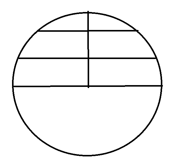
Now do the calculation by integrals: we will use symmetry and only do the upper half and multiply our result by 2. At each  level, call the radius from the center line to the circle
  so the total length of the “y is constant” level is
  and we “multiply by thickness “dy” to obtain
  .
.
But remember that the curve in question is and so if we set  we have
  and so our integral is
Now this integral is no big deal. But HOW we solve it will help us down the road. So here, we use the change of variable (aka “trigonometric substitution”):  to change the integral to:
 therefore
 where:

Yes, I know that this is an easy integral to solve, but I first presented the result this way in order to make a point.
Of course, 
Therefore,  as expected.
Exercise for those seeing this for the first time: compute  and
and  by using the above methods.
Inductive step: Assume  Now calculate using the method of cross sections above (and here we move away from x-y coordinates to more general labeling):

Now we do the substitutions: first of all, we note that  and so
 . Now for the key observation:
  and so
Now use the induction hypothesis to note:

Now do the substitution  and the integral is now:
 which is what we needed to show.
In fact, we have shown a bit more. We’ve shown that  and, in general,

Finishing the formula
We now need to calculate these easy calculus integrals: in this case the reduction formula:
 is useful (it is merely integration by parts). Now use the limits and elementary calculation to obtain:
 to obtain:
 if
if  is even and:
 if is odd.
Now to come up with something resembling a closed formula let’s experiment and do some calculation:
Note that  .
.
So we can make the inductive conjecture that  and see how it holds up:

Now notice the telescoping effect of the fractions from the  factor. All factors cancel except for the
  in the first denominator and the 2 in the first numerator, as well as the
  factor. This leads to:
 as required.
Now we need to calculate 

To simplify this further: split up the factors of the  in the denominator and put one between each denominator factor:
 Now multiply the denominator by
  and put one factor with each
  factor in the denominator; also multiply by in the numerator to obtain:
 Now gather each factor of 2 in the numerator product of the 2k, 2k-2…
 which is the required formula.
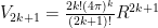
So to summarize:

Note the following:  . If this seems strange at first, think of it this way: imagine the n-ball being “inscribed” in an n-cube which has hyper volume
  . Then consider the ratio
  ; that is, the n-ball holds a smaller and smaller percentage of the hyper volume of the n-cube that it is inscribed in; note the
  corresponds to the number of corners in the n-cube. One might see that the rounding gets more severe as the number of dimensions increases.
One also notes that for fixed radius R,  as well.
There are other interesting aspects to this limit: for what dimension does the maximum hypervolume occur? As you might expect: this depends on the radius involved; a quick glance at the hyper volume formulas will show why. For more on this topic, including an interesting discussion on this limit itself, see Dave Richardson’s blog Division by Zero. Note: his approach to finding the hyper volume formula is also elementary but uses polar coordinate integration as opposed to the method of cross sections.


 but, let’s just say that we aren’t up to differential forms as yet. 🙂