The New Semester: Spring 2014

The new semester is almost upon us here; our classes start up next Wednesday. I am ashamed to report that I am delinquent with a referee’s report; I’ll work some weekends to catch up.

Of course, we come in with “new ideas” which include evaluating things like this:

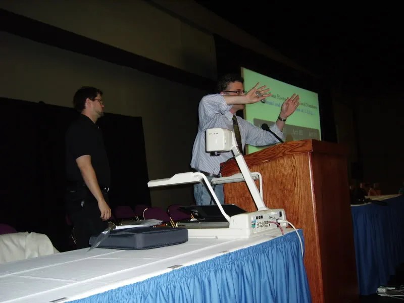
“Most people like to talk about how in college we need to develop critical thinking skills”, said Mike Starbird near the beginning of this talk yesterday, “but really, who wants to hear “Oh, yeah, Soandso, he’s really critical”?”. This, Starbird says, is what led him and coauthor Ed Burger to coin the phrase “effective thinking”. Because that is something one would like to be called.

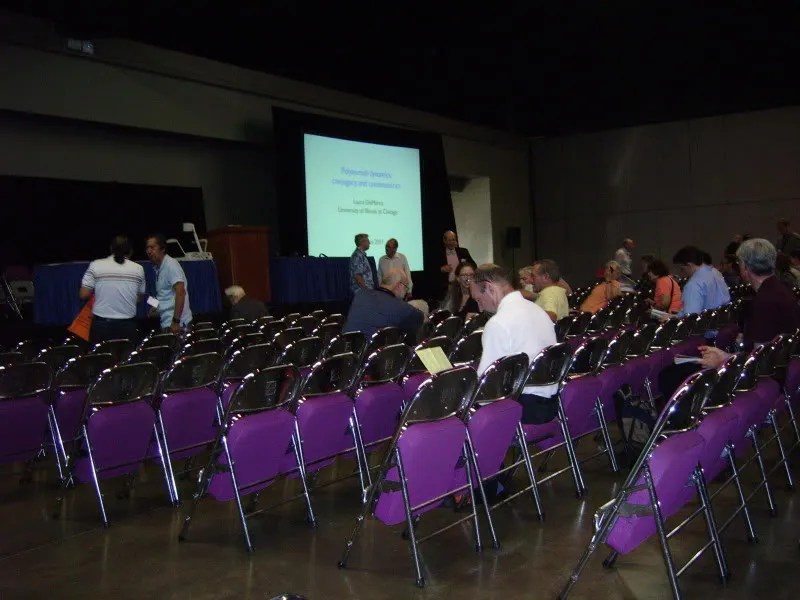
The talk was affected by some technical difficulties, which meant that the slides Starbird had prepared with mathematical examples were unavailable to us. But, following his own advice, Starbird rose to the challenge and gave a talk, without slides, and using the overhead projector for the examples he needed to draw. As usual, his delivery and demeanor were both charming and informative (I am lucky enough to have both taken a class from him and taught a class with him), and the message on what strategies to follow for effective thinking, and to get our own students to be involved in effective thinking, was received loud and clear.

The 5 elements of effective thinking, as Starbird and Burger describe in their eponymous book, are the following: understand simple things deeply, fail to succeed, raise questions, follow the flow of ideas, and everything changes. The first couple he described by using examples of mathematics in which each strategy led to deep insights about a problem. For “understanding simple things deeply”, Starbird showed us a new, purely geometric, way of proving that the derivative of sin(x) is cos(x).

Note: Professor Starbird was one of my professors at the University of Texas. I took a summer class from him which involved the class going over his technical paper called A diagram oriented proof of Dehn’s Lemma

(Roughly speaking: Dehn’s Lemma says that if a polygonal closed curve bounds an immersed polygonal disk whose self intersections lie in the interior of the disk, then that given curve also bounds an embedded polygonal disk (e. g. one without self intersections). Dehn’s Lemma is especially interesting because the first widely accepted “proof” proved to be false; it wasn’t rigorously proved true into years later.)

Ed Burger was a Ph. D. classmate of mine; I consider him a friend. He has won all sorts of awards and is now President of Southwestern University.

I have to chuckle at the goals; at my institution we mostly teach calculus, which is mostly for engineers and scientists. The engineering faculty would blow a gasket if we spent the necessary time for finding deeper proofs that the derivative of sine is cosine.

And yes, we are terribly busy with this or that: on the plate, right off of the bat, is a meeting on “reforming” (read: watering down) our general education program, a visit day, among other things (such as search).

It has gotten to the point to where things like a “department lunch” went from being something fun to do to being “yet another frigging obligation”.

I’ll have to find a way to keep my creative energy up.

So, what I’d like to “think about”:

1. I have a couple of papers out about limits of functions of two variables. Roughly speaking: I gave new proofs of the following:

1. A real valued function of two variables can be continuous when evaluated over all real analytic curves going through the origin and yet still fail to be continuous. (see here)
2. If a real valued function of two variables is continuous when evaluated over all convex functions running through a point, then that function is continuous at that point. This result does NOT extend to .
(see here)

So, what is so special about ? Is this really a theorem about curves through a planar set of points with a limit point? Or is more going on….can this result extend to results about differentiablity?

Then there is something that sparked my interest.

There is this very interesting result about Bezier curves and their control polygons in 3-space: it is known that a Bezzier simple closed curve can be unknotted but have a knotted control polygon. What else is there to explore here? Can only certain differences appear (say, in terms of crossing number or other invariants?) Here is another reference.

I’d like to sink my teeth into this. It doesn’t hurt that I am teaching a numerical methods course. 🙂

In the news….and THINK before you reply to an article. :-)

Ok, a mathematician who is known to be brilliant self-publishes (on the internet) a dense, 512 page proof of a famous conjecture. So what happens?

The Internet exploded. Within days, even the mainstream media had picked up on the story. “World’s Most Complex Mathematical Theory Cracked,” announced the Telegraph. “Possible Breakthrough in ABC Conjecture,” reported the New York Times, more demurely.

On MathOverflow, an online math forum, mathematicians around the world began to debate and discuss Mochizuki’s claim. The question which quickly bubbled to the top of the forum, encouraged by the community’s “upvotes,” was simple: “Can someone briefly explain the philosophy behind his work and comment on why it might be expected to shed light on questions like the ABC conjecture?” asked Andy Putman, assistant professor at Rice University. Or, in plainer words: I don’t get it. Does anyone?

The problem, as many mathematicians were discovering when they flocked to Mochizuki’s website, was that the proof was impossible to read. The first paper, entitled “Inter-universal Teichmuller Theory I: Construction of Hodge Theaters,” starts out by stating that the goal is “to establish an arithmetic version of Teichmuller theory for number fields equipped with an elliptic curve…by applying the theory of semi-graphs of anabelioids, Frobenioids, the etale theta function, and log-shells.”

This is not just gibberish to the average layman. It was gibberish to the math community as well.

[…]

Here is the deal: reading a mid level mathematics research paper is hard work. Refereeing it is even harder work (really checking the proofs) and it is hard work that is not really going to result in anything positive for the person doing the work.

Of course, if you referee for a journal, you do your best because you want YOUR papers to get good refereeing. You want them fairly evaluated and if there is a mistake in your work, it is much better for the referee to catch it than to look like an idiot in front of your community.

But this work was not submitted to a journal. Interesting, no?

Of course, were I to do this, it would be ok to dismiss me as a crank since I haven’t given the mathematical community any reason to grant me the benefit of the doubt.

And speaking of idiots; I made a rather foolish remark in the comments section of this article by Edward Frenkel in Scientific American. The article itself is fine: it is about the Abel prize and the work by Pierre Deligne which won this prize. The work deals with what one might call the geometry of number theory. The idea: if one wants to look for solutions to an equation, say, one gets different associated geometric objects which depend on “what kind of numbers” we allow for . For example, if are integers, we get a 4 point set. If are real numbers, we get a circle in the plane. Then Frenkel remarked:

such as x2 + y2 = 1, we can look for its solutions in different domains: in the familiar numerical systems, such as real or complex numbers, or in less familiar ones, like natural numbers modulo N. For example, solutions of the above equation in real numbers form a circle, but solutions in complex numbers form a sphere.

The comment that I bolded didn’t make sense to me; I did a quick look up and reviewed that actually forms a 3-sphere which lives in . Note: I added in the “absolute value” signs which were not there in the article.

This is easy to see: if then implies that . But that isn’t what was in the article.

Frenkel made a patient, kind response …and as soon as I read “equate real and imaginary parts” I winced with self-embarrassment.

Of course, he admits that the complex version of this equation really yields a PUNCTURED sphere; basically a copy of in .

Just for fun, let’s look at this beast.

Real part of the equation:
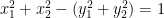
Imaginary part: (for you experts: this is a real algebraic variety in 4-space).

Now let’s look at the intersection of this surface in 4 space with some coordinate planes:
Clearly this surface misses the plane (look at the real part of the equation).
Intersection with the plane yields which is just the unit circle.
Intersection with the plane yields the hyperbola
Intersection with the plane yields the hyperbola
Intersection with the plane yields two isolated points:
Intersection with the plane yields two isolated points:
(so we know that this object is non-compact; this is one reason the “sphere” remark puzzled me)

Science and the media
This Guardian article points out that it is hard to do good science reporting that goes beyond information entertainment. Of course, one of the reasons is that many “groundbreaking” science findings turn out to be false, even if the scientists in question did their work carefully. If this sounds strange, consider the following “thought experiment”: suppose that there are, say, 1000 factors that one can study and only 1 of them is relevant to the issue at hand (say, one place on the genome might indicate a genuine risk factor for a given disease, and it makes sense to study 1000 different places). So you take one at random, run a statistical test at and find statistical significance at . So, if we get a “positive” result from an experiment, what is the chance that it is a true positive? (assume 95 percent accuracy)

So let P represent a positive outcome of a test, N a negative outcome, T means that this is a genuine factor, and F that it isn’t.
Note: P(T) = .001, P(F) = .999, . It follows

So we seek: the probability that a result is true given that a positive test occurred: we seek . That is, given a test is 95 percent accurate, if one is testing for something very rare, there is only about a 2 percent chance that a positive test is from a true factor, even if the test is done correctly!

Mathfest Day III

I only attended the major talks; the first one was by Richard Kenyon. The material, while interesting, flew by a little quickly (though it wouldn’t have for someone who researches full time). The main idea: piecewise approximation to smooth objects is extremely useful, not only topologically but also geometrically (example)

Something especially interesting to me: when trying to approximate certain smooth surfaces, the starting approximation doesn’t matter that much; there are many different piecewise linear sequences that converge to the same surface (not a surprise). There is much more there; this is a lecture I’d like to see again (if it gets posted).

The next one was the third Bernd Sturmfels; this was a continuation of his “algebraic geometry’s usefulness in optimization” series. One big idea: we know how to optimize a linear function on a polygon (e. g., simplex method). It turns out that we can sometimes speed up the process by the “central curve” method; the idea is to use algebraic geometry to do an optimization problem on the constraint plus a term involving logs: form where is the cost function. There is much more there.

The last talk was by an Ivy League professor; it was called “putting topology to work”. On one hand, it was great in the sense that there were many interesting applications. He then asked a sensible question: “how do we teach the essentials of this topology to engineers”?

His solution: revise the undergraduate curriculum so that…well…undergraduates had algebraic topology (or at least homological algebra) in their…linear algebra course. 🙂 It must be nice to teach Ivy league caliber undergraduates. 🙂

The elephant in the room: NO ONE seemed to ask the question: “do the students in our classrooms have the ability to learn this stuff to begin with?”

Do you really think that a class full of students with ACTs in the 22-26 range will be able to EVER handle the advanced stuff, no matter how well it is taught?

Day 2, Madison MAA Mathfest

The day started with a talk by Karen King from the National Council of Teachers of Mathematics.
I usually find math education talks to be dreadful, but this one was pretty good.

The talk was about the importance of future math teachers (K-12) actually having some math background. However, she pointed out that students just having passed math courses didn’t imply that they understood the mathematical issues that they would be teaching…and it didn’t imply that their students would do better.

She gave an example: about half of those seeking to teach high school math couldn’t explain why “division by zero” was undefined! They knew that it was undefined but couldn’t explain why. I found that astonishing since I knew that in high school.

Later, she pointed out that potential teachers with a math degree didn’t understand what the issues were in defining a number like . Of course, a proper definition of this concept requires at least limits or at least a rigorous definition of the log function and she was well aware that the vast majority of high school students aren’t ready for such things. Still, the instructor should be; as she said “we all wave our hands from time to time, but WE should know when we are waving our hands.”

She stressed that we need to get future math teachers to get into the habit (she stressed the word: “habit”) of always asking themselves “why is this true” or “why is it defined in this manner”; too many of our math major courses are rule bound, and at times we write our exams in ways that reward memorization only.

Next, Bernd Sturmfels gave the second talk in his series; this was called Convex Algebraic Geometry.

You can see some of the material here. He also lead this into the concept of “Semidefinite programming”.

The best I can tell: one looks at the objects studied by algebraic geometers (root sets of polynomials of several variables) and then takes a “affine slice” of these objects.

One example: the “n-ellipse” is the set of points on the plane that satisfy where are points in the plane.

Questions: what is the degree of the polynomial that describes the ellipse? What happens if we let tend to zero? What is the smallest for which the ellipse is non-vanishing (Fermat-Webber point)? Note: the 2 ellipse is the circle, the 3 ellipse (degree 8) is what we usually think of as an ellipse.

Note: these type of surfaces can be realized as the determinant of a symmetric matrix; these matrices have real eigenvalues. We can plot curves over which an eigenvalue goes to zero and then changes sign. This process leads to what is known as a spectrahedron ; this is a type of shape in space. A polyhedron can be thought of as the spectrahedron of a diagonal matrix.

Then one can seek to optimize a linear function over a spectrahedron; this leads to semidefinite programming, which, in general, is roughly as difficult as linear programming.

One use: some global optimization problems can be reduced to a semidefinite programming problem (not all).

Shorter Talks
There was a talk by Bob Palais which discussed the role of Rodrigues in the discovery of the quaternions. The idea is that Rodrigues discovered the quaternions before Hamilton did; but he talked about these in terms of rotations in space.

There were a few talks about geometry and how to introduce concepts to students; of particular interest was the concept of a geodesic. Ruth Berger talked about the “fish swimming in jello” model: basically suppose you had a sea of jello where the jello’s density was determined by its depth with the most dense jello (turning to infinite density) at the bottom; and it took less energy for the fish to swim in the less dense regions. Then if a fish wanted to swim between two points, what path would it take? The geometry induced by these geodesics results in the upper half plane model for hyperbolic space.

Nick Scoville gave a talk about discrete Morse theory. Here is a user’s guide. The idea: take a simplicial complex and assign numbers (integers) to the points, segments, triangles, etc. The assignment has to follow rules; basically the boundary of a complex has to have a lower number that what it bounds (with one exception….) and such an assignment leads to a Morse function. Critical sets can be defined and the various Betti numbers can be calculated.

Christopher Frayer then talked about the geometry of cubic polynomials. This is more interesting than it sounds.
Think about this: remember Rolles Theorem from calculus? There is an analogue of this in complex variables called the Guass-Lucas Theorem. Basically, the roots of the derivative lie in the convex hull of the roots of the polynomial. Then there is Marden’s Theorem for polynomials of degree 3. One can talk about polynomials that have a root of and two other roots in the unit circle; then one can study where the the roots of the derivative lie. For a certain class of these polynomials, there is a dead circle tangent to the unit circle at 1 which encloses no roots of the derivative.

MathFest Day Three (Lexington 2011)

I left after the second large lecture and didn’t get a chance to blog about them before now.

But what I saw was very good.

The early lecture was by Lauren Ancel Meyers (Texas-Austin) on Mathematical Approaches to Infectious Disease and Control This is one of those talks where I wish I had access to the slides; they were very useful.

She started out by giving a brief review of the classical SIR model of the spread of a disease which uses the mass action principle (from science) that says that the rate of of change of those infected with a disease is proportional to the product of those who are susceptible to the disease and those who can transmit the disease: . (this actually came from chemistry). Of course, those who are infected either recover or die; this action reduces the number infected. Of course, the number of susceptible also drop.

This leads to a system of differential equations. The basic reproduction number is significant:
where is the recovery rate and is the death rate. Note: if then the disease will die off; if it is greater than 1 we have a pandemic. We can reduce this by reducing (vaccination or quarantine), increasing recovery or, yes, increasing the death rate (as we do with livestock; remember the massive poultry slaughters to stop the spread of flu).

Of course, this model assumes that the infected organisms contact others at random and have equal probabilities of spreading, that the virus doesn’t evolve, etc.

So this model had to be improved on; methods from percolation theory were developed.

So many factors had to be taken into account such as: how much vaccine is there to spread? How far along is the outbreak? (at first children get it; then adults). How severe is the consequences? (we don’t want the virus to evolve to a more dangerous, more resistant form).

Note that the graph model of transmission is dynamic; it can actually change with time.

Of special interest: one can recover the rate of infections of the various strains (and the strains vary from season to season) by looking at the number of times flu related words were searched for on Google. The graph overlap (search rate versus reported cases) was stunning; the only exception is when a scare occurred; then the word search rate lead the actual cases, but that happened only once (2009). Note also that predictions of what will happen get better with a shorter time window (not a surprise).

There was much more in the talk; for example the role of the location of the providers of vaccines was discussed (what is the optimal way to spread out the availability of a given vaccine?)

Manjur Bhargava, Lecture III
First, he noted that in the case where was cubic, that there is always a rational change of variable to put the curve into the following form: where are integers that have the following property: if is any prime where divides then does NOT divide . So this curve can be denoted as .

Also, there are two “generic” cases of curves depending on whether the cubic in has only one real root or three real roots.

This is a catalog of elliptical algebraic curves of the form taken from here. The everywhere smooth curves are considered; the ones with a disconnected graph are said to have “an egg”; those are the ones in which the cubic in has three real roots. In the connected case, the cubic has only one; remember that these are genus one curves; we are seeing a slice of a torus in 4-space (a space with two complex dimensions) in the plane.

Also recall that the rational points on the curve may be finite or infinite. It turns out that the rational points (both coordinates rational) have a group structure (this is called the “divisor class group” in algebraic geometry). This group has a structure that can be understood by a simple geometric construction in the plane, though checking that the operation is associative can be very tedious.

I’ll give a description of the group operation and provide an elementary example:

First, note that if is a point on an elliptical curve, then so is (note: the on the left hand side of the defining equation). That is important. Also note that we will restrict ourselves to smooth curves (that have a well defined tangent line).

The elements of our group will be the rational points of the curve (if any?) along with the point at infinity. If I will denote .

The operation: if are rational points on the curve, construct the line with equation Substitute this into and note that we now have a cubic equation in that has two rational solutions; hence there must be a third rational solution . Associated to that value is two values (possibly double if the value is zero). Call that point on the curve then define where is the reflection of about the axis.

Note the following: that this operation commutes is immediate. If one adds a point to itself, one uses the tangent line as the line through two points; note that such a line might not hit the curve a third time. If such a line is vertical (parallel to the axis) the result is said to be “0” (the point at infinity); if the line is not vertical but still misses the rest of the curve, it is counted three times; that is: . Here are the situations:

Of course, is the group identity. Associativity is difficult to check directly (elementary algebra but very tedious; perhaps 3-4 pages of it?).

Since the group is Abelian, if the group is finite it must be isomorphic to where the second part is the torsion part and the number of infinite cyclic factors is the rank. The rank turns out to be the geometric rank; that is, the minimum number of points required to obtain all of the rational points (infinite number) of the curve. Let be the torsion subgroup; Mazur proved that .

Let’s look at an example of a subgroup of such a curve: let the curve be given by It is easy to see that are all rational points. Let’s see how these work: so this point has order 2. But there is also some interesting behavior: note that which implies that So the tangent line through and are both horizontal; that means that both of these points have order 3. Note also that as the tangent line runs through the point . Similarly So, we can see that have order 6, have order 3 and has order 2. So there is an isomorphism where where the integers are mod 6.

So, we’ve shown a finite Abelian subgroup of the group of rationals of this curve. It turns out that these are the only rational points; here all we get is the torsion group. This curve has rank zero (not obvious).

Note: the group of rationals for is isomorphic to though this isn’t obvious.

The generator of the term is and generates the the torsion term.

History note Some of this was tackled by computers many years ago (Birch, Swinnerton-Dyer). Because computers were so limited in those days, the code had to be very efficient and therefore people had to do quite a bit of work prior to putting it into code; evidently this lead to progress. The speaker joked that such progress might not have been so quickly today due to better computers!

If one looks at where is prime, we should have about points on the curve. So we’d expect that . If there are a lot of rational points on the curve, most of these points would correspond to points. So there is a conjecture by Birch, Swinnerton-Dyer:
where is the rank.

Yes, this is hard; win one million US dollars if you prove it. 🙂

Back to the curves: there are ways of assigning “heights” to these curves; some include:
or

Given this ordering, what are average sizes of ranks?
Katz-Sarnak: half have rank 0, half have rank 1. It was known that average ranks are bounded; previous results had the bound at 2.3, 2, 1.79, assuming that the Generalized Riemann Hypothesis and the Birch, Swinnerton-Dyer conjecture were asssumed.

The speaker and his students got some results without making these large assumptions:

Result 1: when is ordered by height, the average rank is less than 1.
Result 2: A positive portion (10 percent, at least) have rank 0.
Result 3: at least 80 percent have rank 0 or 1.
Corollary: the BSD is true for a positive proportion of elliptic curves;

The speaker (with his student) proved results 1, 2, and 3 and then worked backwards on the existing “BSD true implies X” results to show that BSD was true for a positive proportion of the elliptic curves.

MathFest Day 2 (2011: Lexington, KY)

I went to the three “big” talks in the morning.
Dawn Lott’s talk was about applied mathematics and its relation to the study of brain aneurysms; in particular the aneurysm model was discussed (partial differential equations with a time coordinate and stresses in the radial, circumference and latitudinal directions were modeled).

There was also modeling of the clipping procedure (where the base of the aneurysm was clipped with a metal clip); various clipping strategies were investigated (straight across? diagonal?). One interesting aspect was that the model of the aneurysm was discussed; what shape gave the best results?

Note: this is one procedure that was being modeled:

Next, Bhargava gave his second talk (on rational points on algebraic curves)
It was excellent. In the previous lecture, we saw that a quadratic curve either has an infinite number of rational points or zero rational points. Things are different with a cubic curve.

For example, has exactly one rational point (namely (0,0) ) but has an infinite number! It turns out that the number of rational points an algebraic curve has is related to the genus of the graph of the curve in (where one uses complex values for both variables). The surface is a punctured multi-holed torus of genus with the punctures being “at infinity”.

The genus is as follows: 0 if the degree is 1 or 2, 1 if the degree is 3, and greater than 1 if the degree is 4 or higher. So what about the number of rational points:
0 or finite if the genus is zero
finite if the genus is strictly greater than 1 (Falting’s Theorem; 1983)
indeterminate if the genus is 1. Hence much work is done in this area.

No general algorithm is known to make the determination if the curve is cubic (and therefore of genus 1)

Note: the set of rational points has a group structure.

Note: a rational cubic has a rational change of variable which changes the curve to elliptic form:
Weierstrauss form: where are integers.
Hence this is the form that is studied.
Sometimes the rational points can be found in the following way (example: :
note: this curve is symmetric about the axis.
is a rational point. So is . This line intersects the curve in a third point; this line and the cubic form a cubic in with two rational roots; hence the third must be rational. So we get a third rational point. Then we use to obtain another line and still another rational point; we keep adding rational points in this manner.

This requires proof, but eventually we get all of the rational points in this manner.

The minimum number of “starting points” that we need to find the rational points is called the “rank” of the curve. Our curve is of rank 1 since we really needed only (which, after reflecting, yields a line and a third rational point).

Mordell’s Theorem: every cubic is of finite rank, though it is unknown (as of this time) what the maximum rank is (maximum known example: rank 28), what an expected size would be, or even if “most” are rank 0 or rank 1.

Note: rank 0 means only a finite number of rational points.

Smaller talks
I enjoyed many of the short talks. Of note:
there was a number theory talk by Jay Schiffman in which different conjectures of the following type were presented: if is some sequence of positive integers and we look at the series of partial sums, or partial products (plus or minus some set number), what can we say about the number of primes that we obtain?

Example: Consider the Euclid product of primes (used to show that there is no largest prime number)
etc. It is unknown if there is a largest prime in the sequence .

Another good talk was given by Charlie Smith. It was about the proofs of the irrationality of various famous numbers; it was shown that many of the proofs follow a similar pattern and use a series of 3 techniques/facts that the presenter called “rabbits”. I might talk about this in a later post.

Another interesting talk was given by Jack Mealy. It was about a type of “hyper-hyperbolic” geometry called a “Snell geometry”. Basically one sets up the plane and then puts in a smooth closed boundary curve (say, a line or a sphere). One then declares that the geodesics are those that result from a straight lines…that stay straight until they hit the boundary; they then obey the Snell’s law from physics with respect to the normal of the boundary surface; the two rays joined together from the geodesic in the new geometry. One can do this with, say, a concentric series of circles.

If one arranges the density coefficient in the correct manner, one’s density (in terms of area) can be made to increase as one goes outward; this can lead to interesting area properties of triangles.

Blogging MathFest, 2011 (Lexington, KY)

This is what I am talking about:

I started the day by attending three large lectures:
Laura DeMarco, University of Illinois at Chicago who spoke about dynamical systems (that result from complex polynomials; for example if is a function of the complex plane, one can talk about the orbit of a point . One can then talk about sets of points and This is called the Filled Julia Set.

Ed Burger of Williams (a graduate school classmate of mine who made good) gave the second; he talked about Fibonacci numbers and their relation to irrational ratios (which can be obtained by continued fractions) and various theorems which say that natural numbers can be written uniquely as specified sums of such gadgets.

Lastly Manjul Bhargava of Princeton (who is already full professor though he is less than half my age; he was an Andrew Wiles student) gave a delightful lecture on algebraic curves.

What I noted: all three of these mathematicians are successful enough to be arrogant (especially the third). They could have blown us all away. Yes, they took the time and care to give presentations that actually taught us something.

Of the three, I was the most intrigued by the last one, so I’ll comment on the mathematics.

You’ve probably heard that a Pythagorean triple is a triple of integers such that . For now, we’ll limit ourselves to primitive triples; that is, we’ll assume that have no common factor.

You might have heard that any Pythagorean triple is of the form: for integers. It is true that being defined that way leads to a Pythagorean triple, but why do ALL Pythagorean triples come in this form?

One way to see this is to look at an algebraic curve; in this case, the curve corresponding to . Why? Start with and divide both sides by to obtain One then notes that one is now reduced to looking to rational solutions to (a rational solution to this can be put in the form by getting a common denominator).

We now wish to find all rational points (both coordinates rational) on the circle; clearly is one of them.
Easy claim: if is such a rational point, then the line from to has rational slope.
Not quite as easy claim: if a line running through has rational slope then the line intersects the circle in a rational point.
Verification: such a line has equation and intersects the circle in a point whose value satisfies . This is a quadratic that has rational coefficients and root hence the second root must also be rational. Let’s calculate the second root by doing division: . So the point of intersection has latex and . Both are rational.

Therefore, there is a one to one correspondence between rational slopes and rational points on the circle and all are of the form . Note: we obtain by letting go to infinity; use L’Hopital’s rule on the first coordinate). So if we have any Pythagorean triple then But is rational hence we write where are relatively prime integers. Just a bit of easy algebra reveals which gives us as required.

The point: the algebraic curve motivated the proof that all Pythagorean triples are of that form.

Note: we can extract even more: if latex is any quadratic rational curve (i. e., , all coefficients rational, and is any rational point and there is a line through of rational slope which intersects the curve in a second point (the quadratic nature forbids more than 2 points), the second point must also be rational. This follows by obtaining a quadratic in by substituting and obtaining a quadratic with rational coefficients that has one rational root.

Of course, it might be the case that there is no rational point to choose for . In fact, that is the case for

Why? Suppose there is a rational point on this curve with both fractions in lowest terms. We obtain Now let’s work Mod 4 (hint from the talk): note that in therefore the sum of two squares can only be 0, 1 or 2. The right hand side is either 3 or 0; equality means that both sides are zero. This means that are both even and therefore is divisible by 4 therefore either is even or is even.
Suppose is odd. Then is even and because is even, is even. This contradicts the fact that are relatively prime. If is odd, then because is even, is even. This contradicts the fact that are relatively prime. So both are even which means that are odd. Write where are odd (possibly 1). Then . Now if we obtain on the left hand side (sum of two odd numbers squared) which must be 2 mod 4. The right hand side is still only 3 or 0; this is impossible. Now if, say, then we get which means that the odd number is the difference of two even numbers. That too is impossible.

Hence contains no rational coordinates; that circle manages to miss that dense set.

The point of all of this is that algebraic curves can yield significant information about number theory.

Photos

This is the German Enigma Coding machine (with plug board) at the NSA booth.

This is another view of the Enigma

Edward Burger; I had some bad timing here.

Just prior to the first talk.