College Math Teaching

August 19, 2011

Partial Differential Equations, Differential Equations and the Eigenvalue/Eigenfunction problem

Suppose we are trying to solve the following partial differential equation:
\frac{\partial \psi}{\partial t} = 3 \frac{\partial ^2 \phi}{\partial x^2} subject to boundary conditions:
\psi(0) = \psi(\pi) = 0, \psi(x,0) = x(x-\pi)

It turns out that we will be using techniques from ordinary differential equations and concepts from linear algebra; these might be confusing at first.

The first thing to note is that this differential equation (the so-called heat equation) is known to satisfy a “uniqueness property” in that if one obtains a solution that meets the boundary criteria, the solution is unique. Hence we can attempt to find a solution in any way we choose; if we find it, we don’t have to wonder if there is another one lurking out there.

So one technique that is often useful is to try: let \psi = XT where X is a function of x alone and T is a function of t alone. Then when we substitute into the partial differential equation we obtain:
XT^{\prime} = 3X^{\prime\prime}T which leads to \frac{T^{\prime}}{T} = 3\frac{X^{\prime\prime}}{X}

The next step is to note that the left hand side does NOT depend on x ; it is a function of t alone. The right hand side does not depend on t as it is a function of x alone. But the two sides are equal; hence neither side can depend on x or t ; they must be constant.

Hence we have \frac{T^{\prime}}{T} = 3\frac{X^{\prime\prime}}{X} = \lambda

So far, so good. But then you are told that \lambda is an eigenvalue. What is that about?

The thing to notice is that T^{\prime} - \lambda T = 0 and X^{\prime\prime} - \frac{\lambda}{3}X = 0
First, the equation in T can be written as D(T) = \lambda T with the operator D denoting the first derivative. Then the second can be written as D^2(X) = 3\lambda X where D^2 denotes the second derivative operator. Recall from linear algebra that these operators meet the requirements for a linear transformation if the vector space is the set of all functions that are “differentiable enough”. So what we are doing, in effect, are trying to find eigenvectors for these operators.

So in this sense, solving a homogeneous differential equation is really solving an eigenvector problem; often this is termed the “eigenfucntion” problem.

Note that the differential equations are not difficult to solve:
T = a exp(\lambda T) X  = b exp(\sqrt{\frac{\lambda}{3}} x) + cexp(-\sqrt{\frac{\lambda}{3}} x) ; the real valued form of the equation in x depends on whether \lambda is positive, zero or negative.

But the point is that we are merely solving a constant coefficient differential equation just as we did in our elementary differential equations course with one important difference: we don’t know what the constant (the eigenvalue) is.

Now if we turn to the boundary conditions on x we see that a solution of the form A e^{bx} + Be^{-bx} cannot meet the zero at the boundaries conditions; we can rule out the \lambda = 0 condition as well.
Hence we know that \lambda is negative and we get X = a cos(\sqrt{\frac{\lambda}{3}} x) + b sin(\sqrt{\frac{\lambda}{3}} x) solution and then T = d e^{\lambda t } solution.

But now we notice that these solutions have a \lambda in them; this is what makes these ordinary differential equations into an “eigenvalue/eigenfucntion” problem.

So what values of \lambda will work? We know it is negative so we say \lambda = -w^2 If we look at the end conditions and note that T is never zero, we see that the cosine term must vanish (a = 0 ) and we can ensure that \sqrt{\frac{w}{3}}\pi = k \pi which implies that w = 3k^2 So we get a whole host of functions: \psi_k = a_k e^{-3k^2 t}sin(kx) .

Now we still need to meet the last condition (set at t = 0 ) and that is where Fourier analysis comes in. Because the equation was linear, we can add the solutions and get another solution; hence the X term is just obtained by taking the Fourier expansion for the function x(x-\pi) in terms of sines.

The coefficients are b_k = \frac{1}{\pi} \int^{\pi}_{-\pi} (x)(x-\pi) sin(kx) dx and the solution is:
\psi(x,t) =   \sum_{k=1}^{\infty}  e^{-3k^2 t} b_k sin(kx)

Quantum Mechanics and Undergraduate Mathematics XV: sample problem for stationary states

I feel a bit guilty as I haven’t gone over an example of how one might work out a problem. So here goes:

Suppose our potential function is some sort of energy well: V(x) = 0 for 0 < x < 1 and V(x) = \infty elsewhere.
Note: I am too lazy to keep writing \hbar so I am going with h for now.

So, we have the two Schrödinger equations with \psi being the state vector and \eta_k being one of the stationary states:
-\frac{h^2}{2m} \frac{\partial}{\partial x^2}\eta_k + V(x) \eta_k = ih\frac{\partial}{\partial t} \eta_k
-\frac{h^2}{2m} \frac{\partial}{\partial x^2}\eta_k + V(x) \eta_k = e_k \eta_k

Where e_k are the eigenvalues for \eta_k

Now apply the potential for 0 < x < 1 and the equations become:
-\frac{h^2}{2m} \frac{\partial}{\partial x^2}\eta_k  = ih\frac{\partial}{\partial t} \eta_k
-\frac{h^2}{2m} \frac{\partial}{\partial x^2}\eta_k  = e_k \eta_k

Yes, I know that equation II is a consequence of equation I.

Now we use a fact from partial differential equations: the first equation is really a form of the “diffusion” or “heat” equation; it has been shown that once one takes boundary conditions into account, the equation posses a unique solution. Hence if we find a solution by any means necessary, we don’t have to worry about other solutions being out there.

So attempt a solution of the form \eta_k = X_k T_k where the first factor is a function of x alone and the second is of t alone.
Now put into the second equation:

-\frac{h^2}{2m} X^{\prime\prime}_kT_k  = e_k XT

Now assume T \ne 0 and divide both sides by T and do a little algebra to obtain:
X^{\prime\prime}_k +\frac{2m e_k}{h^2}X_k = 0
e_k are the eigenvalues for the stationary states; assume that these are positive and we obtain:
X = a_k cos(\frac{\sqrt{2m e_k}}{h} x) + b_k sin(\frac{\sqrt{2m e_k}}{h} x)
from our knowledge of elementary differential equations.
Now for x = 0 we have X_k(0) = a_k . Our particle is in our well and we can’t have values below 0; hence a_k = 0 . Now X(x) = b_k sin(\frac{\sqrt{2m e_k}}{h} x)
We want zero at x = 1 so \frac{\sqrt{2m e_k}}{h} = k\pi which means e_k = \frac{(k \pi h)^2}{2m} .

Now let’s look at the first Schrödinger equation:
-\frac{h^2}{2m}X_k^{\prime\prime} T_k = ihT_k^{\prime}X_k
This gives the equation: \frac{X_k^{\prime\prime}}{X_k} = -\frac{ 2m i}{h} \frac{T_k^{\prime}}{T_k}
Note: in partial differential equations, it is customary to note that the left side of the equation is a function of x alone and therefore independent of t and that the right hand side is a function of T alone and therefore independent of x ; since these sides are equal they must be independent of both t and x and therefore constant. But in our case, we already know that \frac{X_k^{\prime\prime}}{X_k} = -2m\frac{e_k}{h^2} . So our equation involving T becomes \frac{T_k^{\prime}}{T_k} = -2m\frac{e_k}{h^2} i \frac{h}{2m} = i\frac{e_k}{h} so our differential equation becomes
T_k {\prime} = i \frac{e_k}{h} T_k which has the solution T_k = c_k exp(i \frac{e_k}{h} t)

So our solution is \eta_k = d_k sin(\frac{\sqrt{2m e_k}}{h} x) exp(i \frac{e_k}{h} t) where e_k = \frac{(k \pi h)^2}{2m} .

This becomes \eta_k = d_k sin(k\pi x) exp(i (k \pi)^2 \frac{\hbar}{2m} t) which, written in rectangular complex coordinates is d_k sin(k\pi x) (cos((k \pi)^2 \frac{\hbar}{2m} t) + i sin((k \pi)^2 \frac{\hbar}{2m} t)

Here are some graphs: we use m = \frac{\hbar}{2} and plot for k = 1, k = 3 and t \in {0, .1, .2, .5} . The plot is of the real part of the stationary state vector.

August 17, 2011

Quantum Mechanics and Undergraduate Mathematics XIV: bras, kets and all that (Dirac notation)

Filed under: advanced mathematics, applied mathematics, linear albegra, physics, quantum mechanics, science — collegemathteaching @ 11:29 pm

Up to now, I’ve used mathematical notation for state vectors, inner products and operators. However, physicists use something called “Dirac” notation (“bras” and “kets”) which we will now discuss.

Recall: our vectors are integrable functions \psi: R^1 \rightarrow C^1 where \int^{-\infty}_{\infty} \overline{\psi} \psi dx converges.

Our inner product is: \langle \phi, \psi \rangle = \int^{-\infty}_{\infty} \overline{\phi} \psi dx

Here is the Dirac notation version of this:
A “ket” can be thought of as the vector \langle , \psi \rangle . Of course, there is an easy vector space isomorphism (Hilbert space isomorphism really) between the vector space of state vectors and kets given by \Theta_k \psi = \langle,\psi \rangle . The kets are denoted by |\psi \rangle .
Similarly there are the “bra” vectors which are “dual” to the “kets”; these are denoted by \langle \phi | and the vector space isomorphism is given by \Theta_b \psi = \langle,\overline{\psi} | . I chose this isomorphism because in the bra vector space, a \langle\alpha,| =  \langle \overline{a} \alpha,| . Then there is a vector space isomorphism between the bras and the kets given by \langle \psi | \rightarrow |\overline{\psi} \rangle .

Now \langle \psi | \phi \rangle is the inner product; that is \langle \psi | \phi \rangle = \int^{\infty}_{-\infty} \overline{\psi}\phi dx

By convention: if A is a linear operator, \langle \psi,|A = \langle A(\psi)| and A |\psi \rangle = |A(\psi) \rangle Now if A is a Hermitian operator (the ones that correspond to observables are), then there is no ambiguity in writing \langle \psi | A | \phi \rangle .

This leads to the following: let A be an operator corresponding to an observable with eigenvectors \alpha_i and eigenvalues a_i . Let \psi be a state vector.
Then \psi = \sum_i \langle \alpha_i|\psi \rangle \alpha_i and if Y is a random variable corresponding to the observed value of A , then P(Y = a_k) = |\langle \alpha_k | \psi \rangle |^2 and the expectation E(A) = \langle \psi | A | \psi \rangle .

August 13, 2011

Beware of Randomness…

Filed under: mathematics education, news, probability, science, statistics — collegemathteaching @ 10:18 pm

We teach about p-values in statistics. But rejecting a null hypothesis at a small p-value does not give us immunity from type I error: (via Scientific American)

The p-value puts a number on the effects of randomness. It is the probability of seeing a positive experimental outcome even if your hypothesis is wrong. A long-standing convention in many scientific fields is that any result with a p-value below 0.05 is deemed statistically significant. An arbitrary convention, it is often the wrong one. When you make a comparison of an ineffective drug to a placebo, you will typically get a statistically significant result one time out of 20. And if you make 20 such comparisons in a scientific paper, on average, you will get one signif­icant result with a p-value less than 0.05—even when the drug does not work.

Many scientific papers make 20 or 40 or even hundreds of comparisons. In such cases, researchers who do not adjust the standard p-value threshold of 0.05 are virtually guaranteed to find statistical significance in results that are meaningless statistical flukes. A study that ran in the February issue of the American Journal
of Clinical Nutrition tested dozens of compounds and concluded that those found in blueberries lower the risk of high blood pressure, with a p-value of 0.03. But the researchers looked at so many compounds and made so many comparisons (more than 50), that it was almost a sure thing that some of the p-values in the paper would be less than 0.05 just by chance.

The same applies to a well-publicized study that a team of neuroscientists once conducted on a salmon. When they presented the fish with pictures of people expressing emotions, regions of the salmon’s brain lit up. The result was statistically signif­icant with a p-value of less than 0.001; however, as the researchers argued, there are so many possible patterns that a statistically significant result was virtually guaranteed, so the result was totally worthless. p-value notwithstanding, there was no way that the fish could have reacted to human emotions. The salmon in the fMRI happened to be dead.

Emphasis mine.

Moral: one can run an experiment honestly and competently and analyze the results competently and honestly…and still get a false result. Damn that randomness!

August 11, 2011

Quantum Mechanics and Undergraduate Mathematics XIII: simplifications and wave-particle duality

In an effort to make the subject a bit more accessible to undergraduate mathematics students who haven’t had much physics training, we’ve made some simplifications. We’ve dealt with the “one dimensional, non-relativistic situation” which is fine. But we’ve also limited ourselves to the case where:
1. state vectors are actual functions (like those we learn about in calculus)
2. eigenvalues are discretely distributed (e. g., the set of eigenvalues have no limit points in the usual topology of the real line)
3. each eigenvalue corresponds to a unique eigenvector.

In this post we will see what trouble simplifications 1 and 2 cause and why they cannot be lived with. Hey, quantum mechanics is hard!

Finding Eigenvectors for the Position Operator
Let X denote the “position” operator and let us seek out the eigenvectors for this operator.
So X\delta = x_0 \delta where \delta is the eigenvector and x_0 is the associated eigenvalue.
This means x\delta = x_0\delta which implies (x-x_0)\delta = 0 .
This means that for x \neq x_0, \delta = 0 and \delta can be anything for x = x_0 . This would appear to allow the eigenvector to be the “everywhere zero except for x_0 ” function. So let \delta be such a function. But then if \psi is any state vector, \int_{-\infty}^{\infty} \overline{\delta}\psi dx = 0 and \int_{-\infty}^{\infty} \overline{\delta}\delta dx = 0 . Clearly this is unacceptable; we need (at least up to a constant multiple) for \int_{-\infty}^{\infty} \overline{\delta}\delta dx = 1

The problem is that restricting our eigenvectors to the class of functions is just too restrictive to give us results; we have to broaden the class of eigenvectors. One way to do that is to allow for distributions to be eigenvectors; the distribution we need here is the dirac delta. In the reference I linked to, one can see how the dirac delta can be thought of as a sort of limit of valid probability density functions. Note: \overline{\delta} = \delta .

So if we let \delta_0 denote the dirac that is zero except for x = x_0 , we recall that \int_{\infty}^{\infty} \delta_0 \psi dx = \psi(x_0) . This means that the probability density function associated with the position operator is P(X = x_0) = |\psi(x_0)|^2

This has an interesting consequence: if we measure the particle’s position at x = x_0 then the state vector becomes \delta_0 . So the new density function based on an immediate measurement of position would be P( X = x_0) = |\langle \delta_0, \delta_0 \rangle|^2 = 1 and P(X = x) = 0 elsewhere. The particle behaves like a particle with a definite “point” position.

Momentum: a different sort of problem

At first the momentum operator P\psi = -i \hbar \frac{d\psi}{dx} seems less problematic. Finding the eigenvectors and eigenfunctions is a breeze: if \theta_0 is the eigenvector with eigenvalue p_0 then:
\frac{d}{dx} \theta_0 = \frac{i}{\hbar}p_0\theta_0 has solution \theta_0 = exp(i p_0 \frac{x}{\hbar}) .
Do you see the problem?

There are a couple of them: first, this provides no restriction on the eigenvalues; in fact the eigenvalues can be any real number. This violates simplification number 2. Secondly, |\theta_0|^2 = 1 therefore |\langle \theta_0, \theta_0 \rangle |^2 = \infty . Our function is far from square integrable and therefore not a valid “state vector” in its present form. This is where the famous “normalization” comes into play.

Mathematically, one way to do this is to restrict the domain (say, limit the non-zero part to x_0 < x < x_1 ) and multiply by an appropriate constant.

Getting back to our state vector: exp(ip_0 \frac{x}{\hbar}) = cos(\frac{p_0 x}{\hbar}) + i sin(\frac{p_0 x}{\hbar}) . So if we measure momentum, we have basically given a particle a wave characteristic with wavelength \frac{\hbar}{p_0} .

Now what about the duality? Suppose we start by measuring a particle’s position thereby putting the state vector in to \psi = \delta_0 . Now what would be the expectation of momentum? We know that the formula is E(P) = -i\hbar \int-{-\infty}^{infty} \delta_0 \frac{\partial \delta_0}{\partial x} dx . But this quantity is undefined because \frac{\partial \delta_0}{\partial x} is undefined.

If we start in a momentum eigenvector and then wish to calculate the position density function (the expectation will be undefined), we see that |\theta_0|^2 = 1 which can be interpreted to mean that any position measurement is equally likely.

Clearly, momentum and position are not compatible operators. So let’s calculate XP - PX
XP \phi = x(-i\hbar \frac{d}{dx} \phi) = -xi\hbar \frac{d}{dx} \phi and PX\phi = -i \hbar\frac{d}{dx} (x \phi) = -i \hbar (\phi + x \frac{d}{dx}\phi) hence (XP - PX)\phi = i\hbar \phi . Therefore XP-PX = i\hbar . Therefore our generalized uncertainty relation tells us \Delta X \Delta P \geq \frac{1}{2}h
(yes, one might object that \Delta X really shouldn’t be defined….) but this uncertainty relation does hold up. So if one uncertainty is zero, then the other must be infinite; exact position means no defined momentum and vice versa.

So: exact, pointlike position means no defined momentum is possible (hence no wave like behavior) but an exact momentum (pure wave) means no exact pointlike position is possible. Also, remember that measurement of position endows a point like state vector of \delta_0 which destroys the wave like property; measurement of momentum endows a wave like state vector \theta_0 and therefore destroys any point like behavior (any location is equally likely to be observed).

Quantum Mechanics and Undergraduate Mathematics XII: position and momentum operators

Filed under: advanced mathematics, applied mathematics, physics, probability, quantum mechanics, science — collegemathteaching @ 1:52 am

Recall that the position operator is X \psi = x\psi and the momentum operator P \psi = -i\hbar \frac{d}{dx} \psi .

Recalling our abuse of notation that said that the expected value E = \langle \psi, A \psi \rangle , we find that the expected value of position is
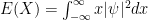
 E(X) = \int_{-\infty}^{\infty} x |\psi|^2 dx . Note: since \int_{-\infty}^{\infty}  |\psi|^2 dx = 1, we can view |\psi|^2 as a probability density function; hence if f is any “reasonable” function of x , then E(f(X)) = \int_{-\infty}^{\infty} f(x) |\psi|^2 dx . Of course we can calculate the variance and other probability moments in a similar way; e. g. E(X^2) =  \int_{-\infty}^{\infty} x |\psi|^2 dx .

Now we turn to momentum; E(P) = \langle \psi, -i\hbar \frac{d}{dx} \psi \rangle = \int_{-\infty}^{\infty} \overline{\psi}\frac{d}{dx}\psi dx and E(P^2) = \langle \psi, P^2\psi \rangle = \langle P\psi, P\psi \rangle = \int_{-\infty}^{\infty} |\frac{d}{dx}\psi|^2 dx

So, back to position: we can now use the fact that |\psi|^2 is a valid density function associated with finding the expected value of position and call this the position probability density function. Hence P(x_1 < x < x_2) = \int_{-\infty}^{\infty} |\psi|^2 dx . But we saw that this can change with time so: P(x_1 < x < x_2; t) = \int_{-\infty}^{\infty} |\psi(x,t)|^2 dx

This is a great chance to practice putting together: differentiation under the integral sign, Schrödinger’s equation and integration by parts. I recommend that the reader try to show:

\frac{d}{dt} \int_{x_1}^{x_2} \overline{\psi}\psi dx = \frac{ih}{2m}(\overline{\psi}\frac{d \psi}{dx}-\psi \frac{d \overline{\psi}}{dx})_{x_1}^{x_2}

The details for the above calculation (students: try this yourself first! 🙂 )

Differentiation under the integral sign:
\frac{d}{dt} \int_{x_1}^{x_2} \overline{\psi} \psi dx = \int_{x_1}^{x_2}\overline{\psi} \frac{\partial \psi}{\partial t} + \psi \frac{\partial \overline{ \psi}}{\partial t} dt

Schrödinger’s equation (time dependent version) with a little bit of algebra:
\frac{\partial \psi}{\partial t} = \frac{i \hbar}{2m} \frac{\partial^2 \psi}{\partial x^2} - \frac{i}{\hbar}V \psi
\frac{\partial \overline{\psi}}{\partial t} = \frac{i \hbar}{2m} \frac{\partial^2 \overline{\psi}}{\partial x^2} + \frac{i}{\hbar}V \overline{\psi}

Note: V is real.

Algebra: eliminate the partial with respect to time terms; multiply the top equation by \overline{\psi} and the second by \psi . Then add the two to obtain:
\overline{\psi} \frac{\partial \psi}{\partial t} + \psi \frac{\partial \overline{ \psi}}{\partial t} = \frac{i \hbar}{2m}(\overline{\psi} \frac{\partial^2 \psi}{\partial x^2} + \psi \frac{\partial^2 \overline{ \psi}}{\partial x^2})

Now integrate by parts:
\frac{i \hbar}{2m} \int_{x_2}^{x_1} (\overline{\psi} \frac{\partial^2 \psi}{\partial x^2} + \psi \frac{\partial^2 \overline{ \psi}}{\partial x^2}) dx =

\frac{ih}{2m} ((\overline{\psi} \frac{\partial \psi}{\partial x})_{x_1}^{x_2} - \int_{x_2}^{x_1} \frac{\partial \overline{\psi}}{\partial x} \frac{\partial \psi}{\partial x} - ( (\psi \frac{\partial \overline{\psi}}{\partial x})_{x_1}^{x_2}  - \int_{x_2}^{x_1}\frac{\partial \psi}{\partial x}\frac{\partial \overline{\psi}}{\partial x}dx)

Now the integrals cancel each other and we obtain our result.

It is common to denote -\frac{ih}{2m}(\overline{\psi}\frac{d \psi}{dx}-\psi \frac{d \overline{\psi}}{dx} by S(x,t) (note the minus sign) and to say \frac{d}{dt}P(x_1 < x < x_2 ; t) = S(x_1,t) - S(x_2,t) (see the reason for the minus sign?)

S(x,t) is called the position probability current at the point x at time t One can think of this as a "probability flow rate" over the point x at time t ; the quantity S(x_1, t) - S(x_2, t) 
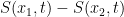
will tell you if the probability of finding the particle between position x_1 and x_2 is going up (positive sign) or down, and by what rate. But it is important that these are position PROBABILITY current and not PARTICLE current; same for |\psi |^2 ; this is the position probability density function, not the particle density function.

NOTE I haven’t talked about the position and momentum eigenvalues or eigenfuctions. We’ll do that in our next post; we’ll run into some mathematical trouble here. No, it won’t be with the position because we already know what a distribution is; the problem is that we’ll find the momentum eigenvector really isn’t square integrable….or even close.

August 10, 2011

Quantum Mechanics and Undergraduate Mathematics XI: an example (potential operator)

Filed under: advanced mathematics, calculus, differential equations, quantum mechanics, science — collegemathteaching @ 8:41 pm

Recall the Schrödinger equations:
-\frac{\hbar^2}{2m} \frac{d^2}{dx^2} \eta_k + V(x) \eta_k = e_k \eta_k and
-\frac{\hbar^2}{2m} \frac{\partial^2}{\partial x^2} \phi + V(x) \phi = i\hbar \frac{\partial}{\partial t}\phi

The first is the time-independent equation which uses the eigenfuctions for the energy operator (Hamiltonian) and the second is the time-dependent state vector equation.

Now suppose that we have a specific energy potential V(x) ; say V(x) = \frac{1}{2}kx^2 . Note: in classical mechanics this follows from Hooke’s law: F(x) = -kx = -\frac{dV}{dx} . In classical mechanics this leads to the following differential equation: ma = m \frac{d^2x}{dt^2} = -kx which leads to \frac{d^2x}{dt^2} + (\frac{k}{m})x = 0 which has general solution x = C_1 sin(wt) +C_2cos(wt) where w = \sqrt{\frac{k}{m}} The energy of the system is given by E = \frac{1}{2}mw^2A^2 where A is the maximum value of x which, of course, is determined by the initial conditions (velocity and displacement at t = 0 ).

Note that there are no a priori restrictions on A . Notation note: A stands for a real number here, not an operator as it has previously.

So what happens in the quantum world? We can look at the stationary states associated with this operator; that means turning to the first Schrödinger equation and substituting V(x) = \frac{1}{2}kx^2 (note k > 0 ):

-\frac{\hbar^2}{2m} \frac{d^2}{dx^2} \eta_k +  \frac{1}{2}kx^2\eta_k = e_k \eta_k

Now let’s do a little algebra to make things easier to see: divide by the leading coefficient and move the right hand side of the equation to the left side to obtain:

\frac{d^2}{dx^2} \eta_k + (\frac{2 e_k m}{(\hbar)^2} - \frac{km}{(\hbar)^2}x^2) \eta_k = 0

Now let’s do a change of variable: let x = rz 
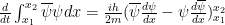
Now we can use the chain rule to calculate: \frac{d^2}{dx^2} = \frac{1}{r^2}\frac{d^2}{dz^2} . Substitution into our equation in x and multiplication on both sides by r^2 yields:
\frac{d^2}{dz^2} \eta_k + (r^2 \frac{2 e_k m}{\hbar^2} - r^4\frac{km}{(\hbar)^2}z^2) \eta_k = 0
Since r is just a real valued constant, we can choose r = (\frac{km}{\hbar^2})^{-1/4} .
This means that r^2 \frac{2 e_k m}{\hbar^2} = \sqrt{\frac{\hbar^2}{km}}\frac{2 e_k m}{(\hbar)^2} = 2 \frac{e_k}{\hbar}\sqrt{\frac{m}{k}}

So our differential equation has been transformed to:
\frac{d^2}{dz^2} \eta_k + (2 \frac{e_k}{\hbar}\sqrt{\frac{m}{k}} - z^2) \eta_k = 0

We are now going to attempt to solve the eigenvalue problem, which means that we will seek values for e_k that yield solutions to this differential equation; a solution to the differential equation with a set eigenvalue will be an eigenvector.

If we were starting from scratch, this would require quite a bit of effort. But since we have some ready made functions in our toolbox, we note 🙂 that setting e_k = (2k+1) \frac{\hbar}{2} \sqrt{{k}{m}} gives us:
\frac{d^2}{dz^2} \eta_k + (2K+1 - z^2) \eta_k = 0

This is the famous Hermite differential equation.

One can use techniques of ordinary differential equations (say, series techniques) to solve this for various values of n .
It turns out that the solutions are:

\eta_k = (-1)^k (2^k k! \sqrt{\pi})^{-1/2} exp(\frac{z^2}{2})\frac{d^k}{dz^k}exp(-z^2) = (2^k k! \sqrt{\pi})^{-1/2} exp(-z^/2)H_k(z) where here H_k(z) is the k'th Hermite polynomial. Here are a few of these:

Graphs of the eigenvectors (in z ) are here:

(graphs from here)

Of importance is the fact that the allowed eigenvalues are all that can be observed by a measurement and that these form a discrete set.

Ok, what about other operators? We will study both the position and the momentum operators, but these deserve their own post as this is where the fun begins! 🙂

Quantum Mechanics and Undergraduate Mathematics X: Schrödinger’s Equations

Filed under: advanced mathematics, applied mathematics, calculus, physics, quantum mechanics, science — collegemathteaching @ 1:19 am

Recall from classical mechanics: E = \frac{1}{2}mv^2 + V(x) where E is energy and V(x) is potential energy. We also have position x and momentum p = mv Note that we can then write E = \frac{p^2}{2m} + V(x) . Analogues exist in quantum mechanics and this is the subject of:

Postulate 6. Momentum and position (one dimensional motion) are represented by the operators:
X = x and P = -i\hbar \frac{d}{dx} respectively. If f is any “well behaved” function of two variables (say, locally analytic?) then A = f(X, P) = f(x, -i\hbar \frac{d}{dx} ) .

To see how this works: let \phi(x) = (2 \pi)^{-\frac{1}{4}}exp(-\frac{x^2}{4})
Then X \phi = (2 \pi)^{-\frac{1}{4}}x exp(-\frac{x^2}{4}) and P \phi = i\hbar (2 \pi)^{-\frac{1}{4}} 2x exp(-\frac{x^2}{4})

Associated with these is energy Hamiltonian operator H = \frac{1}{2m} P^2 + V(X) where P^2 means “do P twice”. So H = -\frac{\hbar^2}{2m}\frac{d^2}{dx^2} + V(x) .

Note We are going to show that these two operators are Hermitian…sort of. Why sort of: these operators A might not be “closed” in the sense that \langle \phi_1, \phi_2 \rangle exists but \langle \phi_1, A \phi_2 \rangle might not exist. Here is a simple example: let \phi_1 = \phi_2 = \sqrt{\frac{2}{\pi} \frac{1}{x^2 + 1}} . Then \langle \phi_1, \phi_2 \rangle = 1 but \int_{-\infty}^{\infty} x \phi_1 dx fails to exist.

So the unstated assumption is that when we are proving that various operators are Hermetian, we mean that they are Hermetian for state vectors which are transformed into functions for which the given inner product is defined.

So, with this caveat in mind, let’s show that these operators are Hermitian.

X clearly is because \langle \phi_1, x \phi_2 \rangle = \langle x \phi_1, \phi_2 \rangle . If this statement is confusing, remember that x is a real variable and therefore \overline{x} = x . Clearly, any well behaved real valued function of x is also a Hermitian operator. IF we assume that P is a Hermitian operator, then \langle \phi_1, P^2 \phi_2 \rangle = \langle P\phi_1, P\phi_2 \rangle = \langle P^2 \phi_1, \phi_2 \rangle . So we must show that P is Hermitian.

This is a nice exercise in integration by parts:
\langle \phi_1, P\phi_2 \rangle = -i\hbar\langle \phi_1, \frac{d}{dx} \phi_2 \rangle = -i\hbar \int_{-\infty}^{\infty} \overline{\phi_1} \frac{d}{dx} \phi_2 dx . Now we note that \overline{\phi_1} \phi_2 |_{-\infty}^{\infty} = 0 (else the improper integrals would fail to converge this is a property assumed for state vectors; mathematically it is possible that the limit as x \rightarrow \infty doesn’t exist but the integral still converges) and so by the integration by parts formula we get i\hbar\int_{-\infty}^{\infty} \overline{\frac{d}{dx}\phi_1}  \phi_2 dx =\int_{-\infty}^{\infty} \overline{-i\hbar\frac{d}{dx}\phi_1}  \phi_2 dx = \langle P\phi_1, \phi_2 \rangle .

Note that potential energy is a function of x so it too is Hermitian. So our Hamiltonian H(p,x) = \frac{1}{2m}P^2 + V(X) = -\frac{h^2}{2m}\frac{d^2}{dx^2} + V(x) is also Hermitian. That has some consequences:

1. H \eta_k = e_k \eta_k
2. H \psi = i\hbar\frac{\partial}{\partial t} \psi

Now we substitute for H and obtain:

1. -\frac{h^2}{2m} \frac{d^2}{dx^2} \eta_k + V(x)\eta_k = e_k \eta_k

2. -\frac{h^2}{2m} \frac{\partial^2}{\partial x^2} \psi + V(x)\psi = i\hbar \frac{\partial}{\partial t} \psi

These are the Schrödinger equations; the first one is the time independent equation. It is about each Hamiltonian energy eigenvector…or you might say each stationary state vector. This holds for each k . The second one is the time dependent one and applies to the state vector in general (not just the stationary states). It is called the fundamental time evolution equation for the state vector.

Special note: if one adjusts the Hamiltonian by adding a constant, the eigenvectors remain the same but the eigenvalues are adjusted by adding a constant. So the adjusted time vector gets adjusted by a factor of exp(-iC \frac{t}{\hbar}) which has a modulus of 1. So the new state vector describes the same state as the old one.

Next post: we’ll give an example and then derive the eigenvalues and eigenvectors for the position and momentum operators. Yes, this means dusting off the dirac delta distribution.

August 9, 2011

Quantum Mechanics and Undergraduate Mathematics IX: Time evolution of an Observable Density Function

We’ll assume a state function \psi and an observable whose Hermitian operator is denoted by A with eigenvectors \alpha_k and eigenvalues a_k . If we take an observation (say, at time t = 0 ) we obtain the probability density function p(Y = a_k) = | \langle \alpha_k, \psi \rangle |^2 (we make the assumption that there is only one eigenvector per eigenvalue).

We saw how the expectation (the expected value of the associated density function) changes with time. What about the time evolution of the density function itself?

Since \langle \alpha_k, \psi \rangle completely determines the density function and because \psi can be expanded as \psi = \sum_{k=1} \langle \alpha_k, \psi \rangle \alpha_k it make sense to determine \frac{d}{dt} \langle \alpha_k, \psi \rangle . Note that the eigenvectors \alpha_k and eigenvalues a_k do not change with time and therefore can be regarded as constants.

\frac{d}{dt} \langle \alpha_k, \psi \rangle =   \langle \alpha_k, \frac{\partial}{\partial t}\psi \rangle = \langle \alpha_k, \frac{-i}{\hbar}H\psi \rangle = \frac{-i}{\hbar}\langle \alpha_k, H\psi \rangle

We can take this further: we now write H\psi = H\sum_j \langle \alpha_j, \psi \rangle \alpha_j = \sum_j \langle \alpha_j, \psi \rangle H \alpha_j We now substitute into the previous equation to obtain:
\frac{d}{dt} \langle \alpha_k, \psi \rangle = \frac{-i}{\hbar}\langle \alpha_k, \sum_j \langle \alpha_j, \psi \rangle H \alpha_j   \rangle = \frac{-i}{\hbar}\sum_j \langle \alpha_k, H\alpha_j \rangle \langle \alpha_j, \psi \rangle

Denote \langle \alpha_j, \psi \rangle by a_j . Then we see that we have the infinite coupled differential equations: \frac{d}{dt} a_k = \frac{-i}{\hbar} \sum_j a_j \langle \alpha_k, H\alpha_j \rangle . That is, the rate of change of one of the a_k depends on all of the a_j which really isn’t a surprise.

We can see this another way: because we have a density function, \sum_j |\langle \alpha_j, \psi \rangle |^2 =1 . Now rewrite: \sum_j |\langle \alpha_j, \psi \rangle |^2 =  \sum_j \langle \alpha_j, \psi \rangle \overline{\langle \alpha_j, \psi \rangle } =  \sum_j a_j \overline{ a_j} = 1 . Now differentiate with respect to t and use the product rule: \sum_j \frac{d}{dt}a_j \overline{ a_j} + a_j  \frac{d}{dt} \overline{ a_j} = 0

Things get a bit easier if the original operator A is compatible with the Hamiltonian H ; in this case the operators share common eigenvectors. We denote the eigenvectors for H by \eta and then
\frac{d}{dt} a_k = \frac{-i}{\hbar} \sum_j a_j \langle \alpha_k, H\alpha_j \rangle becomes:
\frac{d}{dt} \langle \eta_j, \psi \rangle = \frac{-i}{\hbar} \sum_j \langle \eta_j, \psi \rangle \langle \eta_k, H\eta_j \rangle Now use the fact that the \eta_j are eigenvectors for H and are orthogonal to each other to obtain:
\frac{d}{dt} \langle \eta_k, \psi \rangle = \frac{-i}{\hbar} e_k \langle \eta_k, \psi \rangle where e_k is the eigenvalue for H associated with \eta_k .

Now we use differential equations (along with existence and uniqueness conditions) to obtain:
\langle \eta_k, \psi \rangle  = \langle_k, \psi_0 \rangle exp(-ie_k \frac{t}{\hbar}) where \psi_0 is the initial state vector (before it had time to evolve).

This has two immediate consequences:

1. \psi(x,t) = \sum_j \langle \eta_j, \psi_0 \rangle  exp(-ie_j \frac{t}{\hbar}) \eta_j
That is the general solution to the time-evolution equation. The reader might be reminded that exp(ib) = cos(b) + i sin (b)

2. Returning to the probability distribution: P(Y = e_k) = |\langle \eta_k, \psi \rangle |^2 = |\langle \eta_k, \psi_0 \rangle |^2 ||exp(-ie_k \frac{t}{\hbar})|^2 = |\langle \eta_k, \psi_0 \rangle |^2 . But since A is compatible with H , we have the same eigenvectors, hence we see that the probability density function does not change AT ALL. So such an observable really is a “constant of motion”.

Stationary States
Since H is an observable, we can always write \psi(x,t) = \sum_j \langle \eta_j, \psi(x,t) \rangle \eta_j . Then we have \psi(x,t)= \sum_j \langle \eta_j, \psi_0 \rangle exp(-ie_j \frac{t}{\hbar}) \eta_j

Now suppose \psi_0 is precisely one of the eigenvectors for the Hamiltonian; say \psi_0 = \eta_k for some k . Then:

1. \psi_(x,t) = exp(-ie_k \frac{t}{\hbar}) \eta_k
2. For any t \geq 0 , P(Y = e_k) = 1, P(Y \neq  e_k) = 0

Note: no other operator has made an appearance.
Now recall our first postulate: states are determined only up to scalar multiples of unity modulus. Hence the state undergoes NO time evolution, no matter what observable is being observed.

We can see this directly: let A be an operator corresponding to any observable. Then \langle \alpha_k, A \psi_k \rangle = \langle \alpha_k, A exp(-i e_k \frac{t}{\hbar})\eta_k \rangle = exp(-i e_k \frac{t}{\hbar}\langle \alpha_k, A \eta_k \rangle . Then because the probability distribution is completely determined by the eigenvalues e_k and |\langle \alpha_k, A \eta_k \rangle | and |exp(-i e_k \frac{t}{\hbar}| = 1 , the distribution does NOT change with time. This motivates us to define the stationary states of a system: \psi_{(k)} = exp(- e_k \frac{t}{\hbar})\eta_k .

Gillespie notes that much of the problem solving in quantum mechanics is solving the Eigenvalue problem: H \eta_k = e_k \eta_k which is often difficult to do. But if one can do that, one can determine the stationary states of the system.

August 8, 2011

Quantum Mechanics and Undergraduate Mathematics VIII: Time Evolution of Expectation of an Observable

Filed under: advanced mathematics, applied mathematics, physics, probability, quantum mechanics, science — collegemathteaching @ 3:12 pm

Back to our series on QM: one thing to remember about observables: they are operators with a set collection of eigenvectors and eigenvalues (allowable values that can be observed; “quantum levels” if you will). These do not change with time. So \frac{d}{dt} (A (\psi)) = A (\frac{\partial}{\partial t} \psi) . One can work this out by expanding A \psi if one wants to.

So with this fact, lets see how the expectation of an observable evolves with time (given a certain initial state):
\frac{d}{dt} E(A) = \frac{d}{dt} \langle \psi, A \psi \rangle = \langle \frac{\partial}{\partial t} \psi, A \psi \rangle + \langle \psi, A \frac{\partial}{\partial t} \psi \rangle

Now apply the Hamiltonian to account for the time change of the state vector; we obtain:
\langle -\frac{i}{\hbar}H \psi, A \psi \rangle + \langle \psi, -\frac{i}{\hbar}AH \psi \rangle = \overline{\frac{i}{\hbar}} \langle H \psi, A \psi \rangle + -\frac{i}{\hbar} \langle \psi, AH \psi \rangle

Now use the fact that both H and A are Hermitian to obtain:
\frac{d}{dt} A = \frac{i}{\hbar} \langle \psi, (HA - AH) \psi \rangle .
So, we see the operator HA - AH once again; note that if A, H commute then the expectation of the state vector (or the standard deviation for that matter) does not evolve with time. This is certainly true for H itself. Note: an operator that commutes with H is sometimes called a “constant of motion” (think: “total energy of a system in classical mechanics).

Note also that |\frac{d}{dt} A | = |\frac{i}{\hbar} \langle \psi, (HA - AH) \psi \rangle | \leq 2 \Delta A \Delta H

If A does NOT correspond with a constant of motion, then it is useful to define an evolution time T_A = \frac{\Delta A}{\frac{E(A)}{dt}} where \Delta A = (V(A))^{1/2} This gives an estimate of how much time must elapse before the state changes enough to equal the uncertainty in the observable.

Note: we can apply this to H and A to obtain T_A \Delta H \ge \frac{\hbar}{2}

Consequences: if T_A is small (i. e., the state changes rapidly) then the uncertainty is large; hence energy is impossible to be well defined (as a numerical value). If the energy has low uncertainty then T_A must be large; that is, the state is very slowly changing. This is called the time-energy uncertainty relation.

Older Posts »

Blog at WordPress.com.