The purpose of this note is to give a bit of direction to the perplexed student.
I am not going to go into all the possible uses of eigenvalues, eigenvectors, eigenfuntions and the like; I will say that these are essential concepts in areas such as partial differential equations, advanced geometry and quantum mechanics:
Quantum mechanics, in particular, is a specific yet very versatile implementation of this scheme. (And quantum field theory is just a particular example of quantum mechanics, not an entirely new way of thinking.) The states are “wave functions,” and the collection of every possible wave function for some given system is “Hilbert space.” The nice thing about Hilbert space is that it’s a very restrictive set of possibilities (because it’s a vector space, for you experts); once you tell me how big it is (how many dimensions), you’ve specified your Hilbert space completely. This is in stark contrast with classical mechanics, where the space of states can get extraordinarily complicated. And then there is a little machine — “the Hamiltonian” — that tells you how to evolve from one state to another as time passes. Again, there aren’t really that many kinds of Hamiltonians you can have; once you write down a certain list of numbers (the energy eigenvalues, for you pesky experts) you are completely done.
(emphasis mine).
So it is worth understanding the eigenvector/eigenfunction and eigenvalue concept.
First note: “eigen” is German for “self”; one should keep that in mind. That is part of the concept as we will see.
The next note: “eigenfunctions” really are a type of “eigenvector” so if you understand the latter concept at an abstract level, you’ll understand the former one.
The third note: if you are reading this, you are probably already familiar with some famous eigenfunctions! We’ll talk about some examples prior to giving the formal definition. This remark might sound cryptic at first (but hang in there), but remember when you learned  ? That is, you learned that the derivative of
  is a scalar multiple of itself? (emphasis on SELF). So you already know that the function is an eigenfunction of the “operator”
  with eigenvalue
  because that is the scalar multiple.
The basic concept of eigenvectors (eigenfunctions) and eigenvalues is really no more complicated than that. Let’s do another one from calculus:
the function  is an eigenfunction of the operator
  with eigenvalue
  because
  . That is, the function is a scalar multiple of its second derivative. Can you think of more eigenfunctions for the operator ?
Answer:  and are two others, if we only allow for non zero eigenvalues (scalar multiples).
So hopefully you are seeing the basic idea: we have a collection of objects called vectors (can be traditional vectors or abstract ones such as differentiable functions) and an operator (linear transformation) that acts on these objects to yield a new object. In our example, the vectors were differentiable functions, and the operators were the derivative operators (the thing that “takes the derivative of” the function). An eigenvector (eigenfunction)-eigenvalue pair for that operator is a vector (function) that is transformed to a scalar multiple of itself by the operator; e. g., the derivative operator takes to  which is a scalar multiple of the original function.
Formal Definition
We will give the abstract, formal definition. Then we will follow it with some examples and hints on how to calculate.
First we need the setting. We start with a set of objects called “vectors” and “scalars”; the usual rules of arithmetic (addition, multiplication, subtraction, division, distributive property) hold for the scalars and there is a type of addition for the vectors and scalars and the vectors “work together” in the intuitive way. Example: in the set of, say, differentiable functions, the scalars will be real numbers and we have rules such as  , etc. We could also use things like real numbers for scalars, and say, three dimensional vectors such as
 ![[a, b, c]](https://s0.wp.com/latex.php?latex=%5Ba%2C+b%2C+c%5D+&bg=ffffff&fg=000000&s=0&c=20201002) More formally, we start with a vector space (sometimes called a linear space) which is defined as a set of vectors and scalars which obey the vector space axioms.
More formally, we start with a vector space (sometimes called a linear space) which is defined as a set of vectors and scalars which obey the vector space axioms.
Now, we need a linear transformation, which is sometimes called a linear operator. A linear transformation (or operator) is a function  that obeys the following laws:
  and
and  . Note that I am using
  to denote the vectors and the undecorated variable to denote the scalars. Also note that this linear transformation might take one vector space to a different vector space.
Common linear transformations (and there are many others!) and their eigenvectors and eigenvalues.
Consider the vector space of two-dimensional vectors with real numbers as scalars. We can create a linear transformation by matrix multiplication:
![L([x,y]^T) = \left[ \begin{array}{cc} a & b \\ c & d \end{array} \right] \left[ \begin{array}{c} x \\ y \end{array} \right]=\left[ \begin{array}{c} ax+ by \\ cx+dy \end{array} \right]](https://s0.wp.com/latex.php?latex=L%28%5Bx%2Cy%5D%5ET%29+%3D+%5Cleft%5B+%5Cbegin%7Barray%7D%7Bcc%7D+a+%26+b+%5C%5C+c+%26+d+%5Cend%7Barray%7D+%5Cright%5D+%5Cleft%5B+%5Cbegin%7Barray%7D%7Bc%7D+x+%5C%5C+y+%5Cend%7Barray%7D+%5Cright%5D%3D%5Cleft%5B+%5Cbegin%7Barray%7D%7Bc%7D+ax%2B+by+%5C%5C+cx%2Bdy+%5Cend%7Barray%7D+%5Cright%5D++&bg=ffffff&fg=000000&s=0&c=20201002) (note:
(note: ![[x,y]^T](https://s0.wp.com/latex.php?latex=%5Bx%2Cy%5D%5ET+&bg=ffffff&fg=000000&s=0&c=20201002) is the transpose of the row vector; we need to use a column vector for the usual rules of matrix multiplication to apply).
is the transpose of the row vector; we need to use a column vector for the usual rules of matrix multiplication to apply).
It is easy to check that the operation of matrix multiplying a vector on the left by an appropriate matrix is yields a linear transformation.
Here is a concrete example: ![L([x,y]^T) = \left[ \begin{array}{cc} 1 & 2 \\ 0 & 3 \end{array} \right] \left[ \begin{array}{c} x \\ y \end{array} \right]=\left[ \begin{array}{c} x+ 2y \\ 3y \end{array} \right]](https://s0.wp.com/latex.php?latex=L%28%5Bx%2Cy%5D%5ET%29+%3D+%5Cleft%5B+%5Cbegin%7Barray%7D%7Bcc%7D+1+%26+2+%5C%5C+0+%26+3+%5Cend%7Barray%7D+%5Cright%5D+%5Cleft%5B+%5Cbegin%7Barray%7D%7Bc%7D+x+%5C%5C+y+%5Cend%7Barray%7D+%5Cright%5D%3D%5Cleft%5B+%5Cbegin%7Barray%7D%7Bc%7D+x%2B+2y+%5C%5C+3y+%5Cend%7Barray%7D+%5Cright%5D++&bg=ffffff&fg=000000&s=0&c=20201002)
So, does this linear transformation HAVE non-zero eigenvectors and eigenvalues? (not every one does).
Let’s see if we can find the eigenvectors and eigenvalues, provided they exist at all.
For to be an eigenvector for , remember that ![L([x,y]^T) = \lambda [x,y]^T](https://s0.wp.com/latex.php?latex=L%28%5Bx%2Cy%5D%5ET%29+%3D+%5Clambda+%5Bx%2Cy%5D%5ET+&bg=ffffff&fg=000000&s=0&c=20201002) for some real number
for some real number 
So, using the matrix we get: ![L([x,y]^T) = \left[ \begin{array}{cc} 1 & 2 \\ 0 & 3 \end{array} \right] \left[ \begin{array}{c} x \\ y \end{array} \right]= \lambda \left[ \begin{array}{c} x \\ y \end{array} \right]](https://s0.wp.com/latex.php?latex=L%28%5Bx%2Cy%5D%5ET%29+%3D+%5Cleft%5B+%5Cbegin%7Barray%7D%7Bcc%7D+1+%26+2+%5C%5C+0+%26+3+%5Cend%7Barray%7D+%5Cright%5D+%5Cleft%5B+%5Cbegin%7Barray%7D%7Bc%7D+x+%5C%5C+y+%5Cend%7Barray%7D+%5Cright%5D%3D+%5Clambda+%5Cleft%5B+%5Cbegin%7Barray%7D%7Bc%7D+x+%5C%5C+y+%5Cend%7Barray%7D+%5Cright%5D+&bg=ffffff&fg=000000&s=0&c=20201002) . So doing some algebra (subtracting the vector on the right hand side from both sides) we obtain
. So doing some algebra (subtracting the vector on the right hand side from both sides) we obtain ![\left[ \begin{array}{cc} 1 & 2 \\ 0 & 3 \end{array} \right] \left[ \begin{array}{c} x \\ y \end{array} \right] - \lambda \left[ \begin{array}{c} x \\ y \end{array} \right] = \left[ \begin{array}{c} 0 \\ 0 \end{array} \right]](https://s0.wp.com/latex.php?latex=%5Cleft%5B+%5Cbegin%7Barray%7D%7Bcc%7D+1+%26+2+%5C%5C+0+%26+3+%5Cend%7Barray%7D+%5Cright%5D+%5Cleft%5B+%5Cbegin%7Barray%7D%7Bc%7D+x+%5C%5C+y+%5Cend%7Barray%7D+%5Cright%5D+-+%5Clambda+%5Cleft%5B+%5Cbegin%7Barray%7D%7Bc%7D+x+%5C%5C+y+%5Cend%7Barray%7D+%5Cright%5D+%3D+%5Cleft%5B+%5Cbegin%7Barray%7D%7Bc%7D+0+%5C%5C+0+%5Cend%7Barray%7D+%5Cright%5D+&bg=ffffff&fg=000000&s=0&c=20201002)
At this point it is tempting to try to use a distributive law to factor out ![\left[ \begin{array}{c} x \\ y \end{array} \right]](https://s0.wp.com/latex.php?latex=%5Cleft%5B+%5Cbegin%7Barray%7D%7Bc%7D+x+%5C%5C+y+%5Cend%7Barray%7D+%5Cright%5D+&bg=ffffff&fg=000000&s=0&c=20201002) from the left side. But, while the expression makes sense prior to factoring, it wouldn’t AFTER factoring as we’d be subtracting a scalar number from a 2 by 2 matrix! But there is a way out of this: one can then insert the 2 x 2 identity matrix to the left of the second term of the left hand side:
from the left side. But, while the expression makes sense prior to factoring, it wouldn’t AFTER factoring as we’d be subtracting a scalar number from a 2 by 2 matrix! But there is a way out of this: one can then insert the 2 x 2 identity matrix to the left of the second term of the left hand side:
![\left[ \begin{array}{cc} 1 & 2 \\ 0 & 3 \end{array} \right] \left[ \begin{array}{c} x \\ y \end{array} \right] - \lambda\left[ \begin{array}{cc} 1 & 0 \\ 0 & 1 \end{array} \right] \left[ \begin{array}{c} x \\ y \end{array} \right] = \left[ \begin{array}{c} 0 \\ 0 \end{array} \right]](https://s0.wp.com/latex.php?latex=%5Cleft%5B+%5Cbegin%7Barray%7D%7Bcc%7D+1+%26+2+%5C%5C+0+%26+3+%5Cend%7Barray%7D+%5Cright%5D+%5Cleft%5B+%5Cbegin%7Barray%7D%7Bc%7D+x+%5C%5C+y+%5Cend%7Barray%7D+%5Cright%5D+-+%5Clambda%5Cleft%5B+%5Cbegin%7Barray%7D%7Bcc%7D+1+%26+0+%5C%5C+0+%26+1+%5Cend%7Barray%7D+%5Cright%5D+%5Cleft%5B+%5Cbegin%7Barray%7D%7Bc%7D+x+%5C%5C+y+%5Cend%7Barray%7D+%5Cright%5D+%3D+%5Cleft%5B+%5Cbegin%7Barray%7D%7Bc%7D+0+%5C%5C+0+%5Cend%7Barray%7D+%5Cright%5D+&bg=ffffff&fg=000000&s=0&c=20201002)
Notice that by doing this, we haven’t changed anything except now we can factor out that vector; this would leave:
![(\left[ \begin{array}{cc} 1 & 2 \\ 0 & 3 \end{array} \right] - \lambda\left[ \begin{array}{cc} 1 & 0 \\ 0 & 1 \end{array} \right] )\left[ \begin{array}{c} x \\ y \end{array} \right] = \left[ \begin{array}{c} 0 \\ 0 \end{array} \right]](https://s0.wp.com/latex.php?latex=%28%5Cleft%5B+%5Cbegin%7Barray%7D%7Bcc%7D+1+%26+2+%5C%5C+0+%26+3+%5Cend%7Barray%7D+%5Cright%5D++-+%5Clambda%5Cleft%5B+%5Cbegin%7Barray%7D%7Bcc%7D+1+%26+0+%5C%5C+0+%26+1+%5Cend%7Barray%7D+%5Cright%5D+%29%5Cleft%5B+%5Cbegin%7Barray%7D%7Bc%7D+x+%5C%5C+y+%5Cend%7Barray%7D+%5Cright%5D+%3D+%5Cleft%5B+%5Cbegin%7Barray%7D%7Bc%7D+0+%5C%5C+0+%5Cend%7Barray%7D+%5Cright%5D+&bg=ffffff&fg=000000&s=0&c=20201002)
Which leads to:
![(\left[ \begin{array}{cc} 1-\lambda & 2 \\ 0 & 3-\lambda \end{array} \right] ) \left[ \begin{array}{c} x \\ y \end{array} \right] = \left[ \begin{array}{c} 0 \\ 0 \end{array} \right]](https://s0.wp.com/latex.php?latex=%28%5Cleft%5B+%5Cbegin%7Barray%7D%7Bcc%7D+1-%5Clambda+%26+2+%5C%5C+0+%26+3-%5Clambda+%5Cend%7Barray%7D+%5Cright%5D+%29+%5Cleft%5B+%5Cbegin%7Barray%7D%7Bc%7D+x+%5C%5C+y+%5Cend%7Barray%7D+%5Cright%5D+%3D+%5Cleft%5B+%5Cbegin%7Barray%7D%7Bc%7D+0+%5C%5C+0+%5Cend%7Barray%7D+%5Cright%5D+&bg=ffffff&fg=000000&s=0&c=20201002)
Now we use a fact from linear algebra: if is not the zero vector, we have a non-zero matrix times a non-zero vector yielding the zero vector. This means that the matrix is singular. In linear algebra class, you learn that singular matrices have determinant equal to zero. This means that  which means that
  are the respective eigenvalues. Note: when we do this procedure with any 2 by 2 matrix, we always end up with a quadratic with as the variable; if this quadratic has real roots then the linear transformation (or matrix) has real eigenvalues. If it doesn’t have real roots, the linear transformation (or matrix) doesn’t have non-zero real eigenvalues.
Now to find the associated eigenvectors: if we start with  we get
![(\left[ \begin{array}{cc} 0 & 2 \\ 0 & 2 \end{array} \right] \left[ \begin{array}{c} x \\ y \end{array} \right] = \left[ \begin{array}{c} 0 \\ 0 \end{array} \right]](https://s0.wp.com/latex.php?latex=%28%5Cleft%5B+%5Cbegin%7Barray%7D%7Bcc%7D+0+%26+2+%5C%5C+0+%26+2+%5Cend%7Barray%7D+%5Cright%5D++%5Cleft%5B+%5Cbegin%7Barray%7D%7Bc%7D+x+%5C%5C+y+%5Cend%7Barray%7D+%5Cright%5D+%3D+%5Cleft%5B+%5Cbegin%7Barray%7D%7Bc%7D+0+%5C%5C+0+%5Cend%7Barray%7D+%5Cright%5D+&bg=ffffff&fg=000000&s=0&c=20201002) which has solution
which has solution ![\left[ \begin{array}{c} x \\ y \end{array} \right] = \left[ \begin{array}{c} 1 \\ 0 \end{array} \right]](https://s0.wp.com/latex.php?latex=%5Cleft%5B+%5Cbegin%7Barray%7D%7Bc%7D+x+%5C%5C+y+%5Cend%7Barray%7D+%5Cright%5D+%3D+%5Cleft%5B+%5Cbegin%7Barray%7D%7Bc%7D+1+%5C%5C+0+%5Cend%7Barray%7D+%5Cright%5D+&bg=ffffff&fg=000000&s=0&c=20201002) . So that is the eigenvector associated with eigenvalue 1.
. So that is the eigenvector associated with eigenvalue 1.
If we next try  we get
![(\left[ \begin{array}{cc} -2 & 2 \\ 0 & 0 \end{array} \right] \left[ \begin{array}{c} x \\ y \end{array} \right] = \left[ \begin{array}{c} 0 \\ 0 \end{array} \right]](https://s0.wp.com/latex.php?latex=%28%5Cleft%5B+%5Cbegin%7Barray%7D%7Bcc%7D+-2+%26+2+%5C%5C+0+%26+0+%5Cend%7Barray%7D+%5Cright%5D++%5Cleft%5B+%5Cbegin%7Barray%7D%7Bc%7D+x+%5C%5C+y+%5Cend%7Barray%7D+%5Cright%5D+%3D+%5Cleft%5B+%5Cbegin%7Barray%7D%7Bc%7D+0+%5C%5C+0+%5Cend%7Barray%7D+%5Cright%5D+&bg=ffffff&fg=000000&s=0&c=20201002) which has solution
which has solution ![\left[ \begin{array}{c} x \\ y \end{array} \right] = \left[ \begin{array}{c} 1 \\ 1 \end{array} \right]](https://s0.wp.com/latex.php?latex=%5Cleft%5B+%5Cbegin%7Barray%7D%7Bc%7D+x+%5C%5C+y+%5Cend%7Barray%7D+%5Cright%5D+%3D+%5Cleft%5B+%5Cbegin%7Barray%7D%7Bc%7D+1+%5C%5C+1+%5Cend%7Barray%7D+%5Cright%5D+&bg=ffffff&fg=000000&s=0&c=20201002) . So that is the eigenvector associated with the eigenvalue 3.
. So that is the eigenvector associated with the eigenvalue 3.
In the general “k-dimensional vector space” case, the recipe for finding the eigenvectors and eigenvalues is the same.
1. Find the matrix  for the linear transformation.
2. Form the matrix  which is the same as matrix except that you have subtracted from each diagonal entry.
3. Note that  is a polynomial in variable ; find its roots
  . These will be the eigenvalues.
4. Start with  Substitute this into the matrix-vector equation
  and solve for
  . That will be the eigenvector associated with the first eigenvalue. Do this for each eigenvalue, one at a time. Note: you can get up to
  “linearly independent” eigenvectors in this manner; that will be all of them.
Practical note
Yes, this should work “in theory” but practically speaking, there are many challenges. For one: for equations of degree 5 or higher, it is known that there is no formula that will find the roots for every equation of that degree (Galios proved this; this is a good reason to take an abstract algebra course!). Hence one must use a numerical method of some sort. Also, calculation of the determinant involves many round-off error-inducing calculations; hence sometimes one must use sophisticated numerical techniques to get the eigenvalues (a good reason to take a numerical analysis course!)
Consider a calculus/differential equation related case of eigenvectors (eigenfunctions) and eigenvalues.
Our vectors will be, say, infinitely differentiable functions and our scalars will be real numbers. We will define the operator (linear transformation)  , that is, the process that takes the n’th derivative of a function. You learned that the sum of the derivatives is the derivative of the sums and that you can pull out a constant when you differentiate. Hence
  is a linear operator (transformation); we use the term “operator” when we talk about the vector space of functions, but it is really just a type of linear transformation.
We can also use these operators to form new operators; that is  We see that such “linear combinations” of linear operators is a linear operator.
So, what does it mean to find eigenvectors and eigenvalues of such beasts?
Suppose we with to find the eigenvectors and eigenvalues of  . An eigenvector is a twice differentiable function
  (ok, we said “infinitely differentiable”) such that
  or
or  which means
  . You might recognize this from your differential equations class; the only “tweak” is that we don’t know what is. But if you had a differential equations class, you’d recognize that the solution to this differential equation depends on the roots of the characteristic equation
  which has solutions:
  and the solution takes the form
  if the roots are real and distinct,
  if the roots are complex conjugates
  and
and  if there is a real, repeated root. In any event, those functions are the eigenfunctions and these very much depend on the eigenvalues.
Of course, reading this little note won’t make you an expert, but it should get you started on studying.
I’ll close with a link on how these eigenfunctions and eigenvalues are calculated (in the context of solving a partial differential equation).


 ???
??? where
where 
 is finite and that, say,
  is everywhere non-negative and is continuous. Then
  Answer: either zero or it might not exist; in fact, there is no guarantee that
  and we say
  where the overline decoration denotes complex conjugation.
  is finite.
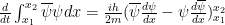
 . This doesn’t seem too hard to do at first, if we use integration by parts:
![\int^{\infty}_{-\infty} \overline{\frac{d^2}{dx^2}\phi} \psi dx = [\overline{\frac{d}{dx}\phi} \psi]^{\infty}_{-\infty} - \int^{\infty}_{-\infty}\overline{\frac{d}{dx}\phi} \frac{d}{dx}\psi dx](https://s0.wp.com/latex.php?latex=%5Cint%5E%7B%5Cinfty%7D_%7B-%5Cinfty%7D+%5Coverline%7B%5Cfrac%7Bd%5E2%7D%7Bdx%5E2%7D%5Cphi%7D+%5Cpsi+dx+%3D+%5B%5Coverline%7B%5Cfrac%7Bd%7D%7Bdx%7D%5Cphi%7D+%5Cpsi%5D%5E%7B%5Cinfty%7D_%7B-%5Cinfty%7D+-+%5Cint%5E%7B%5Cinfty%7D_%7B-%5Cinfty%7D%5Coverline%7B%5Cfrac%7Bd%7D%7Bdx%7D%5Cphi%7D+%5Cfrac%7Bd%7D%7Bdx%7D%5Cpsi+dx+&bg=ffffff&fg=000000&s=0&c=20201002) . Now because the functions are square integrable, the
. Now because the functions are square integrable, the ![[\overline{\frac{d}{dx}\phi} \psi]^{\infty}_{-\infty}](https://s0.wp.com/latex.php?latex=%5B%5Coverline%7B%5Cfrac%7Bd%7D%7Bdx%7D%5Cphi%7D+%5Cpsi%5D%5E%7B%5Cinfty%7D_%7B-%5Cinfty%7D+&bg=ffffff&fg=000000&s=0&c=20201002) term is zero (the functions must go to zero as
term is zero (the functions must go to zero as  tends to infinity) and so we have:
  . Now we use integration by parts again:
![- \int^{\infty}_{-\infty}\overline{\frac{d}{dx}\phi} \frac{d}{dx}\psi dx = -[\overline{\phi} \frac{d}{dx}\psi]^{\infty}_{-\infty} + \int^{\infty}_{-\infty} \overline{\phi}\frac{d^2}{dx^2} \psi dx](https://s0.wp.com/latex.php?latex=-+%5Cint%5E%7B%5Cinfty%7D_%7B-%5Cinfty%7D%5Coverline%7B%5Cfrac%7Bd%7D%7Bdx%7D%5Cphi%7D+%5Cfrac%7Bd%7D%7Bdx%7D%5Cpsi+dx+%3D+-%5B%5Coverline%7B%5Cphi%7D+%5Cfrac%7Bd%7D%7Bdx%7D%5Cpsi%5D%5E%7B%5Cinfty%7D_%7B-%5Cinfty%7D+%2B+%5Cint%5E%7B%5Cinfty%7D_%7B-%5Cinfty%7D+%5Coverline%7B%5Cphi%7D%5Cfrac%7Bd%5E2%7D%7Bdx%5E2%7D+%5Cpsi+dx&bg=ffffff&fg=000000&s=0&c=20201002) which is what we wanted to show.
which is what we wanted to show.  to be square integrable but to be unbounded!
  and base of width
  . Let
. Let ![x \in [k - \frac{1}{2^{3k+1}}, k + \frac{1}{2^{3k+1}}]](https://s0.wp.com/latex.php?latex=x+%5Cin+%5Bk+-+%5Cfrac%7B1%7D%7B2%5E%7B3k%2B1%7D%7D%2C+k+%2B+%5Cfrac%7B1%7D%7B2%5E%7B3k%2B1%7D%7D%5D+&bg=ffffff&fg=000000&s=0&c=20201002) for all positive integers
for all positive integers  has height
  over all of those intervals which means that the area enclosed by each rectangle (tall, but thin rectangles) is
  . Hence
  .
.  and add that to the “square integrable” assumption.
  for
for  and
and  elsewhere.
 so I am going with
  for now.
  being one of the stationary states:

 are the eigenvalues for

 where the first factor is a function of
  alone.
 and divide both sides by
  and do a little algebra to obtain:

 we have
  . Our particle is in our well and we can’t have values below 0; hence
  . Now
. Now 
 so
so  which means
  .
.

 . So our equation involving
  so our differential equation becomes
 which has the solution
 where
where  which, written in rectangular complex coordinates is
 and plot for
  and
and  . The plot is of the real part of the stationary state vector.

 where
where  converges.
 . Of course, there is an easy vector space isomorphism (Hilbert space isomorphism really) between the vector space of state vectors and kets given by
  . The kets are denoted by
  .
. and the vector space isomorphism is given by
  . I chose this isomorphism because in the bra vector space,
  . Then there is a vector space isomorphism between the bras and the kets given by
  .
. is the inner product; that is
 and
and  Now if
  .
. and eigenvalues
  . Let
. Let  and if
  is a random variable corresponding to the observed value of
  and the expectation
  .
. denote the “position” operator and let us seek out the eigenvectors for this operator.
 where
where  is the eigenvector and
  is the associated eigenvalue.
 which implies
  .
. and
and  . This would appear to allow the eigenvector to be the “everywhere zero except for
  and
and  . Clearly this is unacceptable; we need (at least up to a constant multiple) for
 .
. denote the dirac that is zero except for
  . This means that the probability density function associated with the position operator is
 and
and  elsewhere. The particle behaves like a particle with a definite “point” position.
  seems less problematic. Finding the eigenvectors and eigenfunctions is a breeze: if
  is the eigenvector with eigenvalue
  then:
then: has solution
  .
. therefore
  . Our function is far from square integrable and therefore not a valid “state vector” in its present form. This is where the
  ) and multiply by an appropriate constant.
  . So if we measure momentum, we have basically given a particle a wave characteristic with wavelength
  .
.  . Now what would be the expectation of momentum? We know that the formula is
  . But this quantity is undefined because
  is undefined.
 and
and  hence
hence  . Therefore
  . Therefore our generalized uncertainty relation tells us
 really shouldn’t be defined….) but this uncertainty relation does hold up. So if one uncertainty is zero, then the other must be infinite; exact position means no defined momentum and vice versa.
  and the momentum operator
  .
. , we find that the expected value of position is
 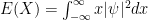 . Note: since
  we can view
  as a probability density function; hence if
  . Of course we can calculate the variance and other probability moments in a similar way; e. g.
  .
. and
and 
 . But we saw that this can change with time so:


 is real.
  and the second by


 by
by  (note the minus sign) and to say
  (see the reason for the minus sign?)
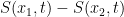 will tell you if the probability of finding the particle between position
  and
and  is going up (positive sign) or down, and by what rate. But it is important that these are position PROBABILITY current and not PARTICLE current; same for
  ; this is the position probability density function, not the particle density function.
  and
and
 ; say
; say  . Note: in classical mechanics this follows from Hooke’s law:
  . In classical mechanics this leads to the following differential equation:
  which leads to
  which has general solution
  where
where  The energy of the system is given by
  where
where  ).
). ):
):

 Now we can use the chain rule to calculate:
  . Substitution into our equation in
  yields:
 is just a real valued constant, we can choose
  .
.

 gives us:
 .
. where here
  is the
  Hermite polynomial. Here are a few of these:
 ) are here:

