Annoying calculations: hypergeometric expectation and variance

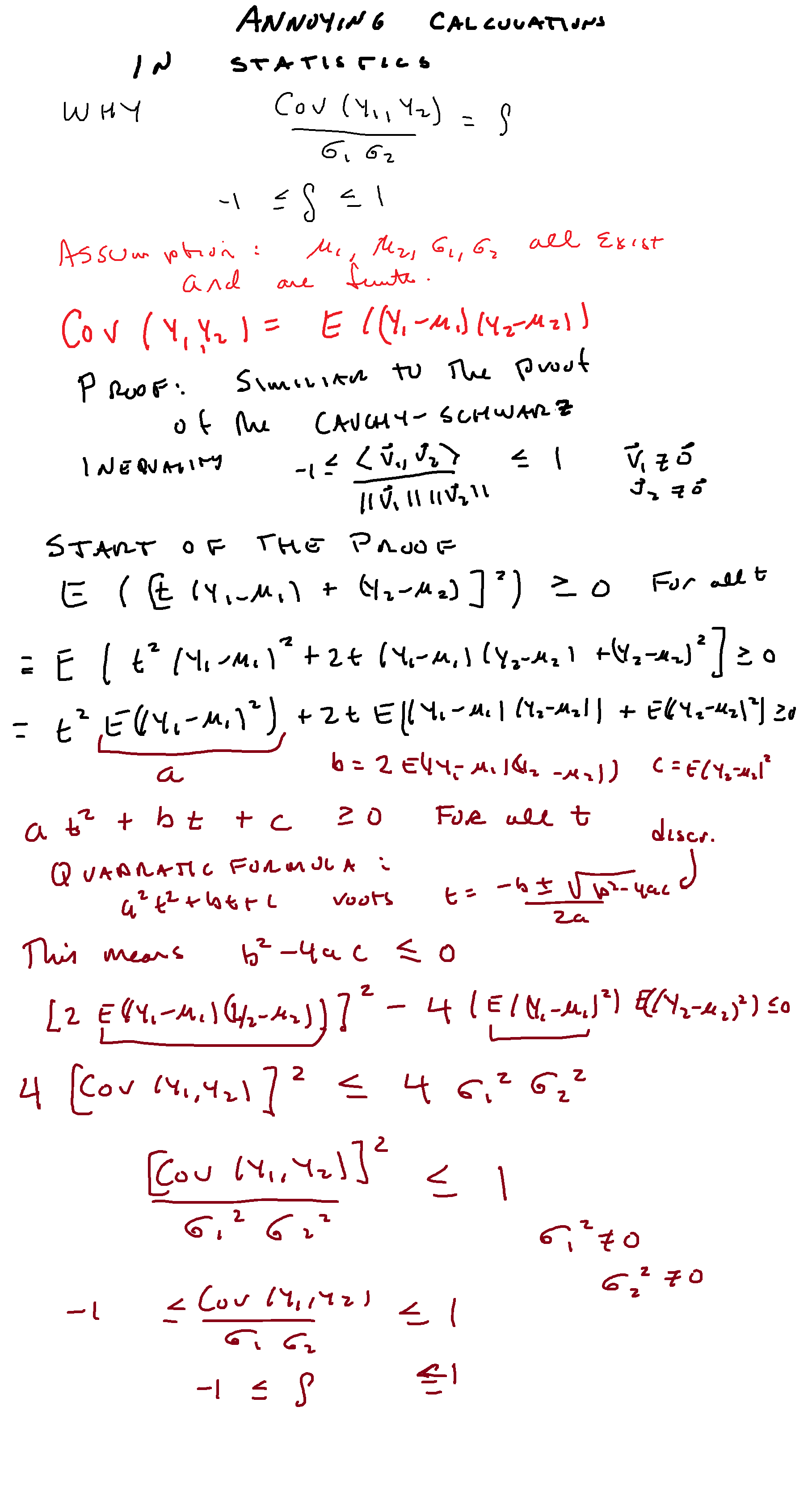
Annoying calculations in Statistics: correlation coefficient is always between -1 and 1.

Yes, I misspelled “Cauchy-Schwarz” in the video.

Annoying calculations: Beta integral

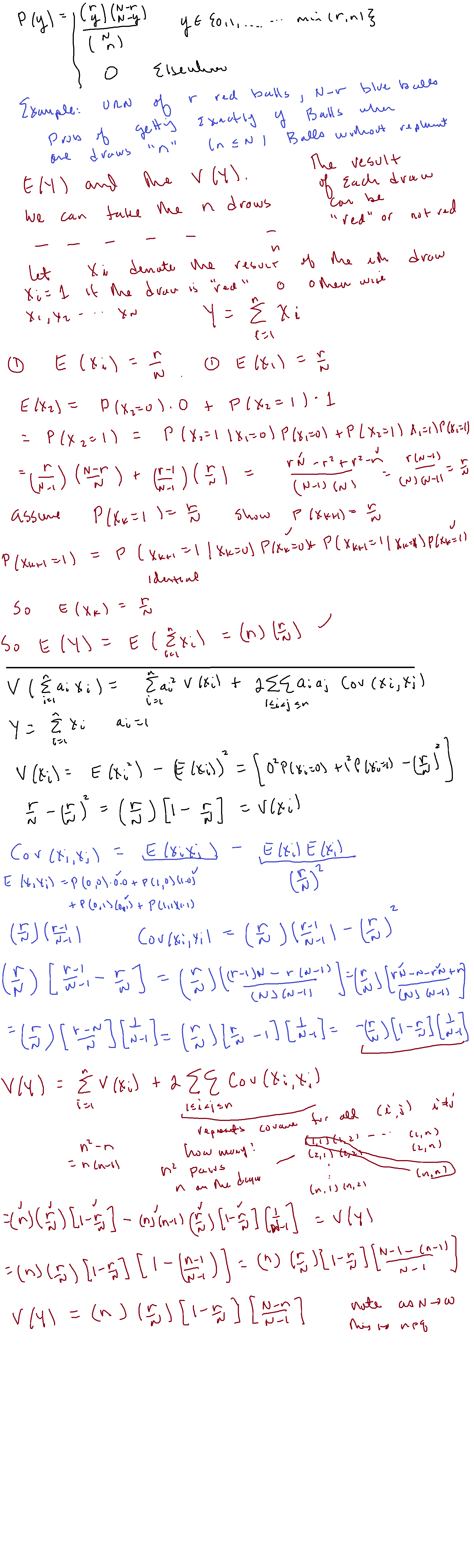
Annoying calculations: Binomial Distribution

Here, we derive the expectation, variance, and moment generating function for the binomial distribution.

Video, when available, will be posted below.

Why the binomial coefficients are integers

The video, when ready, will be posted below.

Vaccine efficacy wrt Hospitalization

I made a short video; no, I did NOT have “risk factor”/”age group” breakdown, but the overall point is that vaccines, while outstanding, are NOT a suit of perfect armor.

Upshot: I used this local data:

The vaccination rate of the area is slightly under 50 percent; about 80 percent for the 65 and up group. But this data doesn’t break it down among age groups so..again, this is “back of the envelope”:

or about 77 percent efficacy with respect to hospitalization, and or 93.75 percent with respect to ending up in the ICU.

Again, the efficacy is probably better than that because of the lack of risk factor correction.

Note: the p-value for the statistical test of vaccines have no effect on hospitalization” vs. “effect” is

The video:

Bayesian Inference: what is it about? A basketball example.

Let’s start with an example from sports: basketball free throws. At a certain times in a game, a player is awarded a free throw, where the player stands 15 feet away from the basket and is allowed to shoot to make a basket, which is worth 1 point. In the NBA, a player will take 2 or 3 shots; the rules are slightly different for college basketball.

Each player will have a “free throw percentage” which is the number of made shots divided by the number of attempts. For NBA players, the league average is .672 with a variance of .0074.

Now suppose you want to determine how well a player will do, given, say, a sample of the player’s data? Under classical (aka “frequentist” ) statistics, one looks at how well the player has done, calculates the percentage () and then determines a confidence interval for said : using the normal approximation to the binomial distribution, this works out to

\

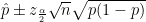
Yes, I know..for someone who has played a long time, one has career statistics ..so imagine one is trying to extrapolate for a new player with limited data.

That seems straightforward enough. But what if one samples the player’s shooting during an unusually good or unusually bad streak? Example: former NBA star Larry Bird once made 71 straight free throws…if that were the sample, with variance zero! Needless to say that trend is highly unlikely to continue.

Classical frequentist statistics doesn’t offer a way out but Bayesian Statistics does.

This is a good introduction:

But here is a simple, “rough and ready” introduction. Bayesian statistics uses not only the observed sample, but a proposed distribution for the parameter of interest (in this case, p, the probability of making a free throw). The proposed distribution is called a prior distribution or just prior. That is often labeled

Since we are dealing with what amounts to 71 Bernoulli trials where p = .672 so the distribution of each random variable describing the outcome of each individual shot has probability mass fuction where for a make and for a miss.

Our goal is to calculate what is known as a posterior distribution (or just posterior) which describes after updating with the data; we’ll call that .

How we go about it: use the principles of joint distributions, likelihood functions and marginal distributions to calculate

The denominator “integrates out” p to turn that into a marginal; remember that the are set to the observed values. In our case, all are 1 with .

What works well is to use the beta distribution for the prior. Note: the pdf is and if one uses , this works very well. Now because the mean will be and given the required mean and variance, one can work out algebraically.

Now look at the numerator which consists of the product of a likelihood function and a density function: up to constant , if we set we get
The denominator: same thing, but gets integrated out and the constant cancels; basically the denominator is what makes the fraction into a density function.

So, in effect, we have which is just a beta distribution with new .

So, I will spare you the calculation except to say that that the NBA prior with leads to

Now the update: .

What does this look like? (I used this calculator)

That is the prior. Now for the posterior:

Yes, shifted to the right..very narrow as well. The information has changed..but we avoid the absurd contention that with a confidence interval of zero width.

We can now calculate a “credible interval” of, say, 90 percent, to see where most likely lies: use the cumulative density function to find this out:

And note that . In fact, Bird’s lifetime free throw shooting percentage is .882, which is well within this 91.6 percent credible interval, based on sampling from this one freakish streak.

The beta function integral: how to evaluate them

My interest in “beta” functions comes from their utility in Bayesian statistics. A nice 78 minute introduction to Bayesian statistics and how the beta distribution is used can be found here; you need to understand basic mathematical statistics concepts such as “joint density”, “marginal density”, “Bayes’ Rule” and “likelihood function” to follow the youtube lecture. To follow this post, one should know the standard “3 semesters” of calculus and know what the gamma function is (the extension of the factorial function to the real numbers); previous exposure to the standard “polar coordinates” proof that would be very helpful.

So, what it the beta function? it is where . Note that for integers The gamma function is the unique “logarithmically convex” extension of the factorial function to the real line, where “logarithmically convex” means that the logarithm of the function is convex; that is, the second derivative of the log of the function is positive. Roughly speaking, this means that the function exhibits growth behavior similar to (or “greater”) than

Now it turns out that the beta density function is defined as follows: for as one can see that the integral is either proper or a convergent improper integral for .

I'll do this in two steps. Step one will convert the beta integral into an integral involving powers of sine and cosine. Step two will be to write as a product of two integrals, do a change of variables and convert to an improper integral on the first quadrant. Then I'll convert to polar coordinates to show that this integral is equal to

Step one: converting the beta integral to a sine/cosine integral. Limit and then do the substitution . Then the beta integral becomes:

Step two: transforming the product of two gamma functions into a double integral and evaluating using polar coordinates.

Write

Now do the conversion to obtain:

(there is a tiny amount of algebra involved)

From which we now obtain

Now we switch to polar coordinates, remembering the that comes from evaluating the Jacobian of

This splits into two integrals:

The first of these integrals is just so now we have:

The second integral: we just use to obtain:

(yes, I cancelled the 2 with the 1/2)

And so the result follows.

That seems complicated for a simple little integral, doesn’t it?

Sign test for matched pairs, Wilcoxon Signed Rank test and Mann-Whitney using a spreadsheet

Our goal: perform non-parametric statistical tests for two samples, both paired and independent. We only assume that both samples come from similar distributions, possibly shifted.

I’ll show the steps with just a bit of discussion of what the tests are doing; the text I am using is Mathematical Statistics (with Applications) by Wackerly, Mendenhall and Scheaffer (7’th ed.) and Mathematical Statistics and Data Analysis by John Rice (3’rd ed.).

First the data: 56 students took a final exam. The professor gave some questions and a committee gave some questions. Student performance was graded and the student performance was graded as a “percent out of 100” on each set of questions (committee graded their own questions, professor graded his questions).

The null hypothesis: student performance was the same on both sets of questions. Yes, this data was close enough to being normal that a paired t-test would have been appropriate and one was done for the committee. But because I am teaching a section on non-parametric statistics, I decided to run a paired sign test and a Wilcoxon signed rank test (and then, for the heck of it, a Mann-Whitney test which assumes independent samples..which these were NOT (of course)). The latter was to demonstrate the technique for the students.

There were 56 exams and “pi” was the score on my questions, “pii” the score on committee questions. The screen shot shows a truncated view.

The sign test for matched pairs.
The idea behind this test: take each pair and score it +1 if sample 1 is larger and score it -1 if the second sample is larger. Throw out ties (use your head here; too many ties means we can’t reject the null hypothesis ..the idea is that ties should be rare).

Now set up a binomial experiment where is the number of pairs. We’d expect that if the null hypothesis is true, where is the probability that the pair gets a score of +1. So the expectation would be and the standard deviation would be , that is,

This is easy to do in a spreadsheet. Just use the difference in rows:

Now use the “sign” function to return a +1 if the entry from sample 1 is larger, -1 if the entry from sample 2 is larger, or 0 if they are the same.

I use “copy, paste, delete” to store the data from ties, which show up very easily.

Now we need to count the number of “+1”. That can be a tedious, error prone process. But the “countif” command in Excel handles this easily.

Now it is just a matter of either using a binomial calculator or just using the normal approximation (I don’t bother with the continuity correction)

Here we reject the null hypothesis that the scores are statistically the same.

Of course, this matched pairs sign test does not take magnitude of differences into account but rather only the number of times sample 1 is bigger than sample 2…that is, only “who wins” and not “by what score”. Clearly, the magnitude of the difference could well matter.

That brings us to the Wilcoxon signed rank test. Here we list the differences (as before) but then use the “absolute value” function to get the magnitudes of such differences.

Now we need to do an “average rank” of these differences (throwing out a few “zero differences” if need be). By “average rank” I mean the following: if there are “k” entries between ranks n, n+1, n+2, ..n+k-1, then each of these gets a rank

(use to work this out).

Needless to say, this can be very tedious. But the “rank.avg” function in Excel really helps.

Example: rank.avg(di, $d$2:$d$55, 1) does the following: it ranks the entry in cell di versus the cells in d2: d55 (the dollar signs make the cell addresses “absolute” references, so this doesn’t change as you move down the spreadsheet) and the “1” means you rank from lowest to highest.

Now the test works in the following manner: if the populations are roughly the same, the larger or smaller ranked differences will each come from the same population roughly half the time. So we denote the sum of the ranks of the negative differences (in this case, where “pii” is larger) and is the sum of the positive differences.

One easy way to tease this out: and can be computed by summing the entries in which the larger differences in “pii” get a negative sign. This is easily done by multiplying the absolute value of the differences by the sign of the differences. Now note that and

One can use a T table (this is a different T than “student T”) or one can use the normal approximation (if n is greater than, say, 25) with
and use the normal approximation.

How these are obtained: the expectation is merely the one half the sum of all the ranks (what one would expect if the distributions were the same) and the variance comes from Bernouilli random variables (one for each pair) with where the variance is

Here is a nice video describing the process by hand:

Mann-Whitney test
This test doesn’t apply here as the populations are, well, anything but independent, but we’ll pretend so we can crunch this data set.

Here the idea is very well expressed:

Do the following: label where the data comes from, and rank it all together. Then add the ranks of the population, of say, the first sample. If the samples are the same, the sums of the ranks should be the same for both populations.

Again, do a “rank average” and yes, Excel can do this over two different columns of data, while keeping the ranks themselves in separate columns.

And one can compare, using either column’s rank sum: the expectation would be and variance would be

Where this comes from: this is really a random sample of since drawn without replacement from a population of integers (all possible ranks…and how they are ordered and the numbers we get). The expectation is and the variance is where (should remind you of the uniform distribution). The rest follows from algebra.

So this is how it goes:

Note: I went ahead and ran the “matched pairs” t-test to contrast with the matched pairs sign test and Wilcoxon test, and the “two sample t-test with unequal variances” to contrast to the Mann-Whitney test..use the “unequal variances” assumption as the variance of sample pii is about double that of pi (I provided the F-test).

An easy fact about least squares linear regression that I overlooked

The background: I was making notes about the ANOVA table for “least squares” linear regression and reviewing how to derive the “sum of squares” equality:

Total Sum of Squares = Sum of Squares Regression + Sum of Squares Error or…

If is the observed response, the sample mean of the responses, and are the responses predicted by the best fit line (simple linear regression here) then:

(where each sum is for the n observations. )

Now for each it is easy to see that but the equations still holds if when these terms are squared, provided you sum them up!

And it was going over the derivation of this that reminded me about an important fact about least squares that I had overlooked when I first presented it.

If you go in to the derivation and calculate:

Which equals and the proof is completed by showing that:

and that BOTH of these sums are zero.

But why?

Let’s go back to how the least squares equations were derived:

Given that

yields that . That is, under the least squares equations, the sum of the residuals is zero.

Now which yields that

That is, the sum of the residuals, weighted by the corresponding x values (inputs) is also zero. Note: this holds with multilinear regreassion as well.

Really, that is what the least squares process does: it sets the sum of the residuals and the sum of the weighted residuals equal to zero.

Yes, there is a linear algebra formulation of this.

Anyhow returning to our sum:

Now for the other term:

Now as it is a constant multiple of the sum of residuals and as it is a constant multiple of the weighted sum of residuals..weighted by the .

That was pretty easy, wasn’t it?

But the role that the basic least squares equations played in this derivation went right over my head!