College Math Teaching

March 14, 2019

Sign test for matched pairs, Wilcoxon Signed Rank test and Mann-Whitney using a spreadsheet

Filed under: statistics, Uncategorized — Tags: , , , — collegemathteaching @ 10:33 pm

Our goal: perform non-parametric statistical tests for two samples, both paired and independent. We only assume that both samples come from similar distributions, possibly shifted.

I’ll show the steps with just a bit of discussion of what the tests are doing; the text I am using is Mathematical Statistics (with Applications) by Wackerly, Mendenhall and Scheaffer (7’th ed.) and Mathematical Statistics and Data Analysis by John Rice (3’rd ed.).

First the data: 56 students took a final exam. The professor gave some questions and a committee gave some questions. Student performance was graded and the student performance was graded as a “percent out of 100” on each set of questions (committee graded their own questions, professor graded his questions).

The null hypothesis: student performance was the same on both sets of questions. Yes, this data was close enough to being normal that a paired t-test would have been appropriate and one was done for the committee. But because I am teaching a section on non-parametric statistics, I decided to run a paired sign test and a Wilcoxon signed rank test (and then, for the heck of it, a Mann-Whitney test which assumes independent samples..which these were NOT (of course)). The latter was to demonstrate the technique for the students.

There were 56 exams and “pi” was the score on my questions, “pii” the score on committee questions. The screen shot shows a truncated view.

The sign test for matched pairs.
The idea behind this test: take each pair and score it +1 if sample 1 is larger and score it -1 if the second sample is larger. Throw out ties (use your head here; too many ties means we can’t reject the null hypothesis ..the idea is that ties should be rare).

Now set up a binomial experiment where n is the number of pairs. We’d expect that if the null hypothesis is true, p = .5 where p is the probability that the pair gets a score of +1. So the expectation would be np = \frac{n}{2} and the standard deviation would be \frac{1}{2} \sqrt{n} , that is, \sqrt{npq}

This is easy to do in a spreadsheet. Just use the difference in rows:

Now use the “sign” function to return a +1 if the entry from sample 1 is larger, -1 if the entry from sample 2 is larger, or 0 if they are the same.

I use “copy, paste, delete” to store the data from ties, which show up very easily.

Now we need to count the number of “+1”. That can be a tedious, error prone process. But the “countif” command in Excel handles this easily.

Now it is just a matter of either using a binomial calculator or just using the normal approximation (I don’t bother with the continuity correction)

Here we reject the null hypothesis that the scores are statistically the same.

Of course, this matched pairs sign test does not take magnitude of differences into account but rather only the number of times sample 1 is bigger than sample 2…that is, only “who wins” and not “by what score”. Clearly, the magnitude of the difference could well matter.

That brings us to the Wilcoxon signed rank test. Here we list the differences (as before) but then use the “absolute value” function to get the magnitudes of such differences.

Now we need to do an “average rank” of these differences (throwing out a few “zero differences” if need be). By “average rank” I mean the following: if there are “k” entries between ranks n, n+1, n+2, ..n+k-1, then each of these gets a rank \frac{n + n+1 + n+2 +...+ n+k-1}{k} = n + \frac{(k-1)}{2}

(use \sum^n_{k=1} k = \frac{n(n+1)}{2} to work this out).

Needless to say, this can be very tedious. But the “rank.avg” function in Excel really helps.

Example: rank.avg(di, $d$2:$d$55, 1) does the following: it ranks the entry in cell di versus the cells in d2: d55 (the dollar signs make the cell addresses “absolute” references, so this doesn’t change as you move down the spreadsheet) and the “1” means you rank from lowest to highest.

Now the test works in the following manner: if the populations are roughly the same, the larger or smaller ranked differences will each come from the same population roughly half the time. So we denote T^{-} the sum of the ranks of the negative differences (in this case, where “pii” is larger) and T^{+} is the sum of the positive differences.

One easy way to tease this out: T^{+} + T^{-1} = \frac{1}{2}n(n+1) and T^{+} - T^{-} can be computed by summing the entries in which the larger differences in “pii” get a negative sign. This is easily done by multiplying the absolute value of the differences by the sign of the differences. Now note that \frac{1}{2}((T^{+} + T^{-1}) + (T^{+} - T^{-1})) = T^{+} and \frac{1}{2}((T^{+} + T^{-1}) - (T^{+} +-T^{-1})) = T^{-}

One can use a T table (this is a different T than “student T”) or one can use the normal approximation (if n is greater than, say, 25) with
E(T^{+})  = \frac{n(n+1)}{2}, V(T^{+})  = \frac{n(n+1)(2n+1)}{24} and use the normal approximation.

How these are obtained: the expectation is merely the one half the sum of all the ranks (what one would expect if the distributions were the same) and the variance comes from n Bernouilli random variables I_k (one for each pair) with p = \frac{1}{2} where the variance is \frac{1}{4} \sum^n_{k=1} k^2 = \frac{1}{4} \frac{n(n+1)(2n+1)}{6}

Here is a nice video describing the process by hand:

Mann-Whitney test
This test doesn’t apply here as the populations are, well, anything but independent, but we’ll pretend so we can crunch this data set.

Here the idea is very well expressed:

Do the following: label where the data comes from, and rank it all together. Then add the ranks of the population, of say, the first sample. If the samples are the same, the sums of the ranks should be the same for both populations.

Again, do a “rank average” and yes, Excel can do this over two different columns of data, while keeping the ranks themselves in separate columns.

And one can compare, using either column’s rank sum: the expectation would be E = \frac{n_1(n_1 +n_2 + 1}{2} and variance would be V = \frac{n_1n_2(n_1+n_2+1)}{12}

Where this comes from: this is really a random sample of since n_1 drawn without replacement from a population of integers 1, 2, ... n_1+n_2 (all possible ranks…and how they are ordered and the numbers we get). The expectation is n_1 \mu and the variance is n_1 \sigma^2 \frac{n_1+n_2-n_1}{n_1+n_2 -1} where \mu = \frac{n_1+n_2 +1}{2}, \sigma^2 \frac{(n_1+n_2)^2-1}{12} (should remind you of the uniform distribution). The rest follows from algebra.

So this is how it goes:

Note: I went ahead and ran the “matched pairs” t-test to contrast with the matched pairs sign test and Wilcoxon test, and the “two sample t-test with unequal variances” to contrast to the Mann-Whitney test..use the “unequal variances” assumption as the variance of sample pii is about double that of pi (I provided the F-test).

January 28, 2015

Prime Ideal Topology

Filed under: Uncategorized — collegemathteaching @ 11:38 am

Note: this is just a watered down version of the Zariski topology on the spectrum of a commutative ring. I got the idea from Steen and Seecbach’s book Counterexamples in Topology.

I am presenting the idea while attempting to use as little ring theory as possible, as some of my students have not had abstract algebra as yet.

Consider the integers Z = \{....-3, -2, -1, 0, 1, 2, 3,... \} . An ideal I is a subset of Z that consists of 0 and all multiples of a given integer. The smallest positive integer k in an ideal is the generator of that ideal; we denote that ideal by (k) .

Examples: (1) =Z since every integer is a multiple of 1, (2) = \{ ...-6, -4, -2, 0, 2, 4, 6, ... \} and (6) = \{ ... -12, -6, 0, 6, 12, 18, ... \} .

An ideal is PRIME if it is generated by a prime number. Now if p is a prime and x \notin (p), y \notin (p) xy \notin (p) because neither has p as a prime factor. So the prime ideals are those ideals whose compliments are multiplicatively closed.

Consider X , the set of prime ideals of Z . That is, X = \{ (0), (2), (3), (5), (7), (11), ... \} The elements (points) of X are prime ideals. Yes, (0) is a prime ideal because if ab  =0 then a = 0 or b = 0 . (1) is not a prime ideal because (1) = Z and a prime ideal cannot be all of Z .

Let’s create a basis for a topology on X : let V_x = \{ I \in X, x \notin I \} . We are indexing subsets of prime ideals by positive integers and zero. Now V_0 = \emptyset as every ideal contains zero. V_1 = X as no prime ideal contains 1 . Now if x \in Z , x has a prime factorization which contains prime factors p_1, p_2, ...p_k , so x \in \cap^k_{i=1} (p_i) so V_x = X -\cup_{i=1}^k (p_i) . That is, the open basis elements are those collections of prime ideals that have a finite complement (those generated by the prime factorization of x .

Examples: V_2 = X - (2), V_8 = X - (2), V_{60} = X - \{(2) \cup (3) \cup (5) \} .

What is a closed set in this topology? A set C \subset X is closed if there exists some ideal I (not necessarily prime) such that C = \{ P \in X | I \subset P \} . For example, C = \{ (2), (3), (5) \} is a closed set because X -C is open. And note (30) \subset (2), (30) \subset (3), (30) \subset (5) . Note: traditionally, the Zariski topology is defined in terms of closed sets.

Clearly a finite union of closed sets is closed and an arbitrary intersection of closed sets is closed.

Now this topology is irreducible, which means that every non-empty pair of open sets intersect as all of them contain (0) . Remember: V_0 = \emptyset as every ideal contains 0. Hence, this topology is not Hausdorff nor is it T_1 ( a topology is T_1 if every two points lie in different open sets, though these sets may intersect each other). This does have the property of being T_0 in that, given two points, there is at least one open set that does not contain both of the points as (p) \notin V_p for p prime.

August 31, 2014

The convolution integral: do some examples in Calculus III or not?

For us, calculus III is the most rushed of the courses, especially if we start with polar coordinates. Getting to the “three integral theorems” is a real chore. (ok, Green’s, Divergence and Stoke’s theorem is really just \int_{\Omega} d \sigma = \int_{\partial \Omega} \sigma but that is the subject of another post)

But watching this lecture made me wonder: should I say a few words about how to calculate a convolution integral?

Note: I’ve discussed a type of convolution integral with regards to solving differential equations here.

In the context of Fourier Transforms, the convolution integral is defined as it was in analysis class: f*g = \int^{\infty}_{-\infty} f(x-t)g(t) dt . Typically, we insist that the functions be, say, L^1 and note that it is a bit of a chore to show that the convolution of two L^1 functions is L^1 ; one proves this via the Fubini-Tonelli Theorem.

(The straight out product of two L^1 functions need not be L^1 ; e.g, consider f(x) = \frac {1}{\sqrt{x}} for x \in (0,1] and zero elsewhere)

So, assuming that the integral exists, how do we calculate it? Easy, you say? Well, it can be, after practice.

But to test out your skills, let f(x) = g(x) be the function that is 1 for x \in [\frac{-1}{2}, \frac{1}{2}] and zero elsewhere. So, what is f*g ???

So, it is easy to see that f(x-t)g(t) only assumes the value of 1 on a specific region of the (x,t) plane and is zero elsewhere; this is just like doing an iterated integral of a two variable function; at least the first step. This is why it fits well into calculus III.

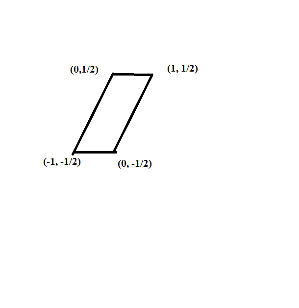
f(x-t)g(t) = 1 for the following region: (x,t), -\frac{1}{2} \le x-t \le \frac{1}{2}, -\frac{1}{2} \le t \le \frac{1}{2}

This region is the parallelogram with vertices at (-1, -\frac{1}{2}), (0, -\frac{1}{2}), (0 \frac{1}{2}), (1, \frac{1}{2}) .

convolutiondraw

Now we see that we can’t do the integral in one step. So, the function we are integrating f(x-t)f(t) has the following description:

f(x-t)f(t)=\left\{\begin{array}{c} 1,x \in [-1,0], -\frac{1}{2} t \le \frac{1}{2}+x \\ 1 ,x\in [0,1], -\frac{1}{2}+x \le t \le \frac{1}{2} \\ 0 \text{ elsewhere} \end{array}\right.

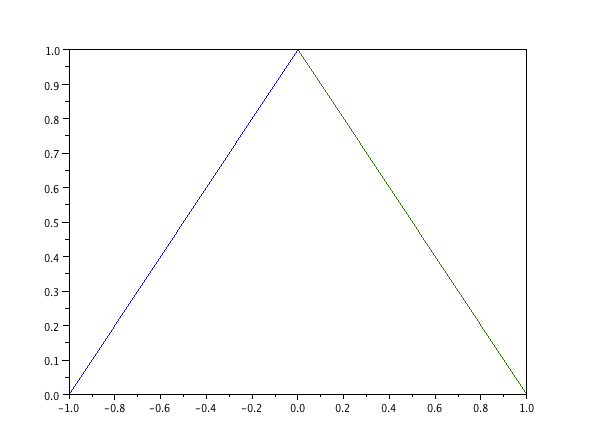
So the convolution integral is \int^{\frac{1}{2} + x}_{-\frac{1}{2}} dt = 1+x for x \in [-1,0) and \int^{\frac{1}{2}}_{-\frac{1}{2} + x} dt = 1-x for x \in [0,1] .

That is, of course, the tent map that we described here. The graph is shown here:

tentmapgraph

So, it would appear to me that a good time to do a convolution exercise is right when we study iterated integrals; just tell the students that this is a case where one “stops before doing the outside integral”.

August 18, 2014

Interchanging infinite sums with integrals

Filed under: Uncategorized — collegemathteaching @ 1:03 pm

This part of this series of lectures got me to thinking about this topic; the relevant part starts at 13 minutes:

(side note: I am enjoying these and hope to finish all 30!)

Of interest here: if u(x,t) describes the heat in a one dimensional circle of metal and the radius is one, one can do the analysis of the heat equation u_t = a u_{xx} with initial condition u(x,0) = f(x) and assuming that u has a Fourier expansion (complex coefficients) one can obtain: u(x,t) = \Sigma_k \hat{f_k}e^{-4ak \pi^2t}e^{2k \pi i x} which can be rewritten as \Sigma_k (\int^1_0 f(w) e^{-2k \pi i w} dw) e^{-4ak \pi^2t}e^{2k \pi i x} = \Sigma_k (\int^1_0 f(w) e^{-2k \pi i (x-w)} ) e^{-4ak \pi^2t} dw . Note: k ranges from -\infty to \infty and by \Sigma^{\infty}_{k=-\infty} c_k we mean lim_{n \rightarrow \infty} \Sigma^{n}_{k=-n}c_k and note that c_k, c_{-k} are complex conjugates for all k .

Now IF we could interchange the summation sign and the integral sign we’d have: \int^1_0 \Sigma_k f(w) e^{-2k \pi i (x-w)}  e^{-4ak \pi^2t} dw . Now let g(x,t) = e^{-2k \pi i (x)}  e^{-4ak \pi^2t} then we could say that u(x,t) = \int^1_0 g(x-w,t) f(w) dw which is a convolution product; g(x,t) is the heat kernel which is a nice form. But about that interchange: when can we do it?

First note that by \Sigma_k f_k we mean the limit of the sequence of partial sums: \phi_n = \Sigma_{k = -n}^{n} f_k and if \int^1_0 lim_n \phi_n = lim_n \int^1_0 \phi_n then the interchange is valid. NOTE: I am following the custom of not using the “differential” dx and of letting it be understood that lim_n means lim_{n \rightarrow \infty} .

The “I don’t want “TL;DR” answer” version
If you are comfortable with Lebesgue integration, then the Dominated Convergence Theorem is the standard: if \phi_n are all measurable functions and lim_n \phi_n = \phi (pointwise) and there exists an integrable function g where g \ge |\phi_n| for all n , then \int^1_0 lim_n \phi_n = lim_n \int^1_0 \phi_n = \int^1_0 \phi .

Now if the terms “Lebesgue integration” and “measurable” has you scratching your head, you can either learn a bit about it or, if you are in the “tl;dr” mode I’ll make some (hopefully) “practitioner friendly” remarks.

First of all, all Riemann integrable functions are Lebesgue integrable (provided we are NOT talking about improper integrals) and a “measurable function” is one in which the inverse image of a “measurable set” is a “measurable set”. Now “measurable set”: these include sets that single point sets, open intervals, closed intervals, countable intersections of such, countable unions of such and complements of such unions and intersections. Unfortunately there are measurable sets that aren’t formed in this manner, and there are such things as non-measurable sets. See here for the definition of “measurable set”.

Upshot: the sort of functions that appear in Fourier Series are measurable so you probably don’t have to worry. So there is probably no harm in assuming that the \phi_n are Riemann integrable functions.

Pointwise convergence: this means for all x in the domain of interest (here, x \in [0,1] ), lim \phi_n(x) = \phi(x) .

Of course, when we are talking about the Fourier series for a given function f , there are conditions that must be met to get that the the series converges to a function that is “almost f ; the video assumes that f is L_2 which means that \int^1_0 (f)^2 exists. The mathematics of convergence of a Fourier series is rich; for this note we will assume that the Fourier series in question converges.

Now for the conclusion: assuming that the \phi_n converge pointwise to some \phi then lim_n \int^1_0 \phi_n = \int^1_0 lim_n \phi_n but we need to use the Lebesgue integral to guarantee this equality..in general. This is why:

For example, suppose we enumerate the rational numbers by q_{1},q_{2},...q_{k}... and define f_{1}(x)=\left\{\begin{array}{c}1,x\neq q_{1} \\ 0,x=q_{1}\end{array}\right. and then inductively define f_{k}(x)=\left\{\begin{array}{c}1,x\notin \{q_{1},q_{2},..q_{k}\} \\ 0,x\in \{q_{1},q_{2},..q_{k}\}\end{array}\right.  . Then f_{k}\rightarrow f=\left\{\begin{array}{c}1,x\notin \{q_{1},q_{2},..q_{k}....\} \\ 0,x\in \{q_{1},q_{2},..q_{k},...\}\end{array}\right. and for each k, \int_{0}^{1}f_{k}(x)dx=1 but f, the limit function, is not Riemann integrable. It is Lebesgue integrable though, and the integral remains 1.

But, given the types of series that the practitioner will be working with (typically: only a finite number of maximums and minimums on a given interval and a finite number of jump discontinuities), one will probably not encounter such pathological behavior with the functions. I give this example to explain why the Dominated Convergence Theorem uses Lebesgue integrals.

Wait a minute you might say, didn’t I read something about “uniform convergence” of functions that lead to the limiting behavior that we need? Well, yes, and I’ll explain that here:

we say that \phi_n \rightarrow \phi uniformly if for any \epsilon  > 0 there exists N such that for all n  > N , |\phi_n(x) - \phi(x)|  < 0 for ALL x  in the interval of interest. Then, it a routine exercise in Riemann integration to see that if \phi_n \rightarrow \phi uniformly then \int^1_0 \phi_n \rightarrow \int^1_0 \phi . The down side is that we rarely have uniform convergence when we are talking about Fourier series terms. Here is why: it is known that if \phi_n \rightarrow \phi uniformly and that if all of the \phi_n are continuous, then the limit function \phi is continuous as well. However when one obtains the Fourier series for a function with jump discontinuities (say, for a pulse wave) one sees that the terms (and hence the sequence of partial sums) of the Fourier series are continuous but what the Fourier series converges to is not continuous; hence the convergence of the series is NOT uniform.

January 22, 2014

Mean Value Theorem for integrals and it’s use in Taylor Polynomial approximations

Filed under: Uncategorized — collegemathteaching @ 3:12 am

First, what is the Mean Value Theorem for integrals? There are two common versions (calculus level versions; one can make these more general):

Version one: if f is continuous over [a,b] then there is some c \in (a,b) such that f(c)(b-a) = \int^b_a f(x) dx . The proof is pretty easy: Let F(t) = \int^t_af(x)dx then the Fundamental Theorem of Calculus says that F is continuous on [a,b] and differentiable on (a,b) so the Mean Value Theorem applies: there is some c \in (a,b) where F'(c)=f(x) =\frac{F(b)-F(a)}{b-a} = \frac{1}{b-a} \int^b_a f(x)dx and the result follows.

This version has a nice geometric interpretation. If one interprets the definite integral as an area bounded by the graph of the function, the x axis and the lines x=a, x =b then the Mean Value Theorem says that there is a rectangle whose base is b-a and whose height is f(c) whose area is equal to the integral.

mvtintegrals

But there is a second version:

Version Two: if f is continuous over [a,b] and g is positive and continuous (actually, integrable and positive is enough) on [a,b] then there is some c \in (a,b) where f(c)\int^b_a g(x) dx = \int^b_a f(x) g(x) dx .

The proof of this result is not much harder than the first one. Since f is continuous over [a,b] , f attains both a maximum and a minimum value on the interval; say the maximum is f(x_M) is the maximum; f(x_m) is the minimum. So we have for all x \in [a,b], f(x_m)g(x) \le f(x)g(x) \le f(x_M)g(x) Now integrate: f(x_m)\int^b_ag(x)dx \le \int^b_af(x)g(x)dx \le f(x_M)\int^b_ag(x)dx Now divide through by \int^b_a g(x) dx  and note that the integral is positive. So f(x_m) \le \frac{\int^b_af(x)g(x)dx}{\int^b_a g(x) dx} \le f(x_M) . Now because f is continuous, every value between f(x_m), f(x_M) is attained by f so there is at least one c such that f(c) = \frac{\int^b_af(x)g(x)dx}{\int^b_a g(x) dx} and the result follows.

So, what does this have to do with Taylor polynomials?

In a previous post we went over how to use integration by parts to obtain a Taylor polynomial for a function that has a sufficient number of derivatives. Here is the plan:

for our purposes, let f have as many derivatives at 0 as desired.

Now compute \int^x_0f'(t)dt = f(x)-f(0) . Now compute by using integration by parts: u =f'(t), dv= dt, du =f"(t), v = t-x (if the assignment of v seems strange, remember we can use ANY anti-derivative of dv .)

So we have f'(t)(t-x)|^x_0 - \int^x_0 f"(t)(t-x)dt = f(x)-f(0) so by substitution we obtain f(0)+f'(0)x - \int^x_0 f"(t)(t-x) dt =f(x)

I’ll repeat the process so you can see what happens to the sign in front of the integral: we use parts again: u =f"(t), dv = (t-x), du = f^{(3)}(t), v = \frac{1}{2}(t-x)^2 and so we obtain (for the integral) \frac{1}{2}f"(t)(t-x)^2|^x_0 -\frac{1}{2}\int^x_0 f^{(3)}(t)(t-x)^2dt =-\frac{1}{2}f"(0)x^2-\frac{1}{2}\int^x_0 f^{(3)}(t)(t-x)^2dt Now substitute this for the integral in the order 1 expression, and remember the negative sign: we obtain f(0)+f'(0)x \frac{1}{2}f"(0)x^2+\frac{1}{2}\int^x_0 f^{(3)}(t)(t-x)^2dt =f(x)

So we can proceed inductively; the important thing here is the remainder term after n steps is \pm \frac{1}{n!} \int^x_0 f^{(n+1)}(t)(t-x)^n dt

A word on the sign: the negative occurs when n is odd and positive when n is even. So one can remove this ambiguity by replacing (t-x) by (x-t) and so the remainder formula becomes: \frac{1}{n!} \int^x_0 f^{(n+1)}(t)(x-t)^n dt .

Now this is still not the usual Lagrange or Cauchy remainder formula that many texts give. But we can get that from our Mean Value Theorem for integrals. Since the integrand is continuous over the interval [0,x] the First Mean Value Theorem for Integrals says that there exists a \zeta \in (0,x) where \frac{1}{n!}f^{(n+1)}(\zeta)x(x-\zeta)^n  is the remainder; that is the Cauchy form.

The Lagrange form comes from the Second Mean Value Theorem for Integrals: we know that there is a \omega \in (0,x) where \frac{1}{n!} \int^x_0 f^{(n+1)}(t)(x-t)^n dt = f^{(n+1)}(\omega)\frac{1}{n!}\int^x_0(x-t)^n dt = \frac{1}{(n+1)!}f^{(n+1)}(\omega)x^{(n+1)}

That is the Lagrange version of the error term that one usually sees.

December 21, 2013

Rant: please stop with the teaching of “gimmicks for calculation”

Filed under: calculus, editorial, integrals, student learning, Uncategorized — Tags: — collegemathteaching @ 1:05 pm

I finished teaching calculus II (our course: techniques for integration, applications of integrals and infinite sequences/series) and noticed that some of our freshmen students came in knowing how to do many of the calculations…did well on the first exam…then didn’t do so well in the rest of the course.

Evidently, they were well versed in calculation tricks learned in high school; give them \int x^3 sin(x) dx and they could whip out a table.

So here is my rant: we teach integration by parts not so much to calculate integrals like \int x^3 sin(x) dx (which can be rapidly done with a calculator) but rather so they can understand the technique of integration by parts.

Why? Well, there are many uses of integration by parts and I’ll just display a few uses of them:

1. Taylor Polynomials. How do we get these? If we assume that f has enough derivatives, we proceed in the following manner: calculate \int ^x_0 f'(t) dt in two different ways: use the Fundamental Theorem of calculus on one side (to obtain f(x) - f(0) and use integration by parts on the other side: u = f'(t), dv = dt, du = f''(t), v = t-x (yes, we are being choosy about which anti derivative of dv to use).
This means: -\int^x_0 f''(t)(t-x)dt +f'(t)(t-x)|^x_0 = f(x)-f(0) so f(x) = f(0) + f'(0)x -\int^x_0 f''(t)(t-x)dt =f(x) and one proceeds from there.

2. Differential equations: given y' + p(x)y = f(x) one seeks to find an integrating factor (which is e^{\int p(x)} so as to get:

e^{\int p(x)}y' + p(x)e^{\int p(x)}y = f(x)e^{\int p(x)} which can be written as \frac{d}{dx}(e^{\int p(x)}y) = f(x)e^{\int p(x)}. That is, the left hand side is just the product rule for derivatives, which, as you know (if you are a calculus teacher), is really all integration by parts is!

Sure, one can jazz it up (as we subtly did in the Taylor Polynomial calculation); the integration by parts formula is really \frac{d}{dx} (f(x)g(x)) = \frac{d}{dx}(f(x)+ C) g(x) + f(x)\frac{d}{dx}(g(x) + D) where C, D are arbitrary constants. But, my main point is that integration by parts should be UNDERSTOOD; short cuts to do tedious calculations are relatively unimportant, IMHO.

Now if you want to ask students “why does tabular integration work”, then….GREAT!

December 30, 2012

2012 in review

Filed under: Uncategorized — collegemathteaching @ 10:33 pm

The WordPress.com stats helper monkeys prepared a 2012 annual report for this blog.

Here’s an excerpt:

600 people reached the top of Mt. Everest in 2012. This blog got about 11,000 views in 2012. If every person who reached the top of Mt. Everest viewed this blog, it would have taken 18 years to get that many views.

Click here to see the complete report.

May 26, 2012

Eigenvalues, Eigenvectors, Eigenfunctions and all that….

The purpose of this note is to give a bit of direction to the perplexed student.

I am not going to go into all the possible uses of eigenvalues, eigenvectors, eigenfuntions and the like; I will say that these are essential concepts in areas such as partial differential equations, advanced geometry and quantum mechanics:

Quantum mechanics, in particular, is a specific yet very versatile implementation of this scheme. (And quantum field theory is just a particular example of quantum mechanics, not an entirely new way of thinking.) The states are โ€œwave functions,โ€ and the collection of every possible wave function for some given system is โ€œHilbert space.โ€ The nice thing about Hilbert space is that itโ€™s a very restrictive set of possibilities (because itโ€™s a vector space, for you experts); once you tell me how big it is (how many dimensions), youโ€™ve specified your Hilbert space completely. This is in stark contrast with classical mechanics, where the space of states can get extraordinarily complicated. And then there is a little machine โ€” โ€œthe Hamiltonianโ€ โ€” that tells you how to evolve from one state to another as time passes. Again, there arenโ€™t really that many kinds of Hamiltonians you can have; once you write down a certain list of numbers (the energy eigenvalues, for you pesky experts) you are completely done.

(emphasis mine).

So it is worth understanding the eigenvector/eigenfunction and eigenvalue concept.

First note: “eigen” is German for “self”; one should keep that in mind. That is part of the concept as we will see.

The next note: “eigenfunctions” really are a type of “eigenvector” so if you understand the latter concept at an abstract level, you’ll understand the former one.

The third note: if you are reading this, you are probably already familiar with some famous eigenfunctions! We’ll talk about some examples prior to giving the formal definition. This remark might sound cryptic at first (but hang in there), but remember when you learned \frac{d}{dx} e^{ax} = ae^{ax} ? That is, you learned that the derivative of e^{ax} is a scalar multiple of itself? (emphasis on SELF). So you already know that the function e^{ax} is an eigenfunction of the “operator” \frac{d}{dx} with eigenvalue a because that is the scalar multiple.

The basic concept of eigenvectors (eigenfunctions) and eigenvalues is really no more complicated than that. Let’s do another one from calculus:
the function sin(wx) is an eigenfunction of the operator \frac{d^2}{dx^2} with eigenvalue -w^2 because \frac{d^2}{dx^2} sin(wx) = -w^2sin(wx). That is, the function sin(wx) is a scalar multiple of its second derivative. Can you think of more eigenfunctions for the operator \frac{d^2}{dx^2} ?

Answer: cos(wx) and e^{ax} are two others, if we only allow for non zero eigenvalues (scalar multiples).

So hopefully you are seeing the basic idea: we have a collection of objects called vectors (can be traditional vectors or abstract ones such as differentiable functions) and an operator (linear transformation) that acts on these objects to yield a new object. In our example, the vectors were differentiable functions, and the operators were the derivative operators (the thing that “takes the derivative of” the function). An eigenvector (eigenfunction)-eigenvalue pair for that operator is a vector (function) that is transformed to a scalar multiple of itself by the operator; e. g., the derivative operator takes e^{ax} to ae^{ax} which is a scalar multiple of the original function.

Formal Definition
We will give the abstract, formal definition. Then we will follow it with some examples and hints on how to calculate.

First we need the setting. We start with a set of objects called “vectors” and “scalars”; the usual rules of arithmetic (addition, multiplication, subtraction, division, distributive property) hold for the scalars and there is a type of addition for the vectors and scalars and the vectors “work together” in the intuitive way. Example: in the set of, say, differentiable functions, the scalars will be real numbers and we have rules such as a (f + g) =af + ag , etc. We could also use things like real numbers for scalars, and say, three dimensional vectors such as [a, b, c] More formally, we start with a vector space (sometimes called a linear space) which is defined as a set of vectors and scalars which obey the vector space axioms.

Now, we need a linear transformation, which is sometimes called a linear operator. A linear transformation (or operator) is a function L that obeys the following laws: L(\vec{v} + \vec{w}) = L(\vec{v}) + L(\vec{w} ) and L(a\vec{v}) = aL(\vec{v}) . Note that I am using \vec{v} to denote the vectors and the undecorated variable to denote the scalars. Also note that this linear transformation L might take one vector space to a different vector space.

Common linear transformations (and there are many others!) and their eigenvectors and eigenvalues.
Consider the vector space of two-dimensional vectors with real numbers as scalars. We can create a linear transformation by matrix multiplication:

L([x,y]^T) = \left[ \begin{array}{cc} a & b \\ c & d \end{array} \right] \left[ \begin{array}{c} x \\ y \end{array} \right]=\left[ \begin{array}{c} ax+ by \\ cx+dy \end{array} \right]  (note: [x,y]^T is the transpose of the row vector; we need to use a column vector for the usual rules of matrix multiplication to apply).

It is easy to check that the operation of matrix multiplying a vector on the left by an appropriate matrix is yields a linear transformation.
Here is a concrete example: L([x,y]^T) = \left[ \begin{array}{cc} 1 & 2 \\ 0 & 3 \end{array} \right] \left[ \begin{array}{c} x \\ y \end{array} \right]=\left[ \begin{array}{c} x+ 2y \\ 3y \end{array} \right]

So, does this linear transformation HAVE non-zero eigenvectors and eigenvalues? (not every one does).
Let’s see if we can find the eigenvectors and eigenvalues, provided they exist at all.

For [x,y]^T to be an eigenvector for L , remember that L([x,y]^T) = \lambda [x,y]^T for some real number \lambda

So, using the matrix we get: L([x,y]^T) = \left[ \begin{array}{cc} 1 & 2 \\ 0 & 3 \end{array} \right] \left[ \begin{array}{c} x \\ y \end{array} \right]= \lambda \left[ \begin{array}{c} x \\ y \end{array} \right] . So doing some algebra (subtracting the vector on the right hand side from both sides) we obtain \left[ \begin{array}{cc} 1 & 2 \\ 0 & 3 \end{array} \right] \left[ \begin{array}{c} x \\ y \end{array} \right] - \lambda \left[ \begin{array}{c} x \\ y \end{array} \right] = \left[ \begin{array}{c} 0 \\ 0 \end{array} \right]

At this point it is tempting to try to use a distributive law to factor out \left[ \begin{array}{c} x \\ y \end{array} \right] from the left side. But, while the expression makes sense prior to factoring, it wouldn’t AFTER factoring as we’d be subtracting a scalar number from a 2 by 2 matrix! But there is a way out of this: one can then insert the 2 x 2 identity matrix to the left of the second term of the left hand side:
\left[ \begin{array}{cc} 1 & 2 \\ 0 & 3 \end{array} \right] \left[ \begin{array}{c} x \\ y \end{array} \right] - \lambda\left[ \begin{array}{cc} 1 & 0 \\ 0 & 1 \end{array} \right] \left[ \begin{array}{c} x \\ y \end{array} \right] = \left[ \begin{array}{c} 0 \\ 0 \end{array} \right]

Notice that by doing this, we haven’t changed anything except now we can factor out that vector; this would leave:
(\left[ \begin{array}{cc} 1 & 2 \\ 0 & 3 \end{array} \right]  - \lambda\left[ \begin{array}{cc} 1 & 0 \\ 0 & 1 \end{array} \right] )\left[ \begin{array}{c} x \\ y \end{array} \right] = \left[ \begin{array}{c} 0 \\ 0 \end{array} \right]

Which leads to:

(\left[ \begin{array}{cc} 1-\lambda & 2 \\ 0 & 3-\lambda \end{array} \right] ) \left[ \begin{array}{c} x \\ y \end{array} \right] = \left[ \begin{array}{c} 0 \\ 0 \end{array} \right]

Now we use a fact from linear algebra: if [x,y]^T is not the zero vector, we have a non-zero matrix times a non-zero vector yielding the zero vector. This means that the matrix is singular. In linear algebra class, you learn that singular matrices have determinant equal to zero. This means that (1-\lambda)(3-\lambda) = 0 which means that \lambda = 1, \lambda = 3 are the respective eigenvalues. Note: when we do this procedure with any 2 by 2 matrix, we always end up with a quadratic with \lambda as the variable; if this quadratic has real roots then the linear transformation (or matrix) has real eigenvalues. If it doesn’t have real roots, the linear transformation (or matrix) doesn’t have non-zero real eigenvalues.

Now to find the associated eigenvectors: if we start with \lambda = 1 we get
(\left[ \begin{array}{cc} 0 & 2 \\ 0 & 2 \end{array} \right]  \left[ \begin{array}{c} x \\ y \end{array} \right] = \left[ \begin{array}{c} 0 \\ 0 \end{array} \right] which has solution \left[ \begin{array}{c} x \\ y \end{array} \right] = \left[ \begin{array}{c} 1 \\ 0 \end{array} \right] . So that is the eigenvector associated with eigenvalue 1.
If we next try \lambda = 3 we get
(\left[ \begin{array}{cc} -2 & 2 \\ 0 & 0 \end{array} \right]  \left[ \begin{array}{c} x \\ y \end{array} \right] = \left[ \begin{array}{c} 0 \\ 0 \end{array} \right] which has solution \left[ \begin{array}{c} x \\ y \end{array} \right] = \left[ \begin{array}{c} 1 \\ 1 \end{array} \right] . So that is the eigenvector associated with the eigenvalue 3.

In the general “k-dimensional vector space” case, the recipe for finding the eigenvectors and eigenvalues is the same.
1. Find the matrix A for the linear transformation.
2. Form the matrix A - \lambda I which is the same as matrix A except that you have subtracted \lambda from each diagonal entry.
3. Note that det(A - \lambda I) is a polynomial in variable \lambda ; find its roots \lambda_1, \lambda_2, ...\lambda_n . These will be the eigenvalues.
4. Start with \lambda = \lambda_1 Substitute this into the matrix-vector equation det(A - \lambda I) \vec{v_1} = \vec{0} and solve for \vec({v_1} . That will be the eigenvector associated with the first eigenvalue. Do this for each eigenvalue, one at a time. Note: you can get up to k “linearly independent” eigenvectors in this manner; that will be all of them.

Practical note
Yes, this should work “in theory” but practically speaking, there are many challenges. For one: for equations of degree 5 or higher, it is known that there is no formula that will find the roots for every equation of that degree (Galios proved this; this is a good reason to take an abstract algebra course!). Hence one must use a numerical method of some sort. Also, calculation of the determinant involves many round-off error-inducing calculations; hence sometimes one must use sophisticated numerical techniques to get the eigenvalues (a good reason to take a numerical analysis course!)

Consider a calculus/differential equation related case of eigenvectors (eigenfunctions) and eigenvalues.
Our vectors will be, say, infinitely differentiable functions and our scalars will be real numbers. We will define the operator (linear transformation) D^n = \frac{d^n}{dx^n} , that is, the process that takes the n’th derivative of a function. You learned that the sum of the derivatives is the derivative of the sums and that you can pull out a constant when you differentiate. Hence D^n is a linear operator (transformation); we use the term “operator” when we talk about the vector space of functions, but it is really just a type of linear transformation.

We can also use these operators to form new operators; that is (D^2 + 3D)(y) = D^2(y) + 3D(y) = \frac{d^2y}{dx^2} + 3\frac{dy}{dx} We see that such “linear combinations” of linear operators is a linear operator.

So, what does it mean to find eigenvectors and eigenvalues of such beasts?

Suppose we with to find the eigenvectors and eigenvalues of (D^2 + 3D) . An eigenvector is a twice differentiable function y (ok, we said “infinitely differentiable”) such that (D^2 + 3D) = \lambda y or \frac{d^2y}{dx^2} + 3\frac{dy}{dx} = \lambda y which means \frac{d^2y}{dx^2} + 3\frac{dy}{dx} - \lambda y = 0 . You might recognize this from your differential equations class; the only “tweak” is that we don’t know what \lambda is. But if you had a differential equations class, you’d recognize that the solution to this differential equation depends on the roots of the characteristic equation m^2 + 3m - \lambda = 0 which has solutions: m = -\frac{3}{2} \pm \frac{\sqrt{9-4\lambda}}{2} and the solution takes the form e^{m_1}, e^{m_2} if the roots are real and distinct, e^{ax}sin(bx), e^{ax}cos(bx) if the roots are complex conjugates a \pm bi and e^{m}, xe^{m} if there is a real, repeated root. In any event, those functions are the eigenfunctions and these very much depend on the eigenvalues.

Of course, reading this little note won’t make you an expert, but it should get you started on studying.

I’ll close with a link on how these eigenfunctions and eigenvalues are calculated (in the context of solving a partial differential equation).

March 6, 2010

The Principle of Mathematical Induction: why it works

Filed under: induction, logic, transfinite induction, Uncategorized — collegemathteaching @ 11:03 pm

For those who prefer a video:

I am writing this post because I’ve seen that there is some misunderstanding of what mathematical induction is and why it works.

  • What is mathematical induction? It is a common proof technique. Basically, if one wants to show that a statement is true in generality and that one can index the set of statements via the integers (or by some other appropriate index set), then one can use induction.Here is a common example: suppose one wants to show that

    1 + 2 + 3 + ....+ k = (1/2)*(k)*(k+1) for all positive integers k
    (for example, 1 + 2 + 3 + 4 + 5 = (1/2)*(5)*(5+1) = 15 ).

    Initial step: 1 = (1/2)*(1)*(1+1)= 1 so the statement is true for k = 1 .

    Inductive step: assume that the formula holds for some integer k .
    Finish the proof: show that if the formula holds for some integer k , then it holds for k+1 as well.

    So 1 + 2 + 3 +....+ k + (k+1) = (1 + 2 + ...+ k) + (k+1) =(1/2)*(k)*(k+1) + (k + 1)
    (why? because we assumed that k was an integer for which
    1 + 2 + 3 + ....+ k = (1/2)*(k)*(k+1) . )

    so 1 + 2 + 3 +....+ k + (k+1) = (1/2)*(k)*(k+1) + (k + 1) = ((1/2)*k + 1)*(k+1) (factor out a k+1 term)
    = (1/2)*2*((1/2)*k + 1)*(k+1) = (1/2)*(k+2)*(k+1)=(1/2)*(k+1)*(k+2)=(1/2)*(k+1)*(k+1 + 1)
    which is what we needed to show. So the proof would be done.

  • Why does induction “prove” anything? Mathematical induction is equivalent to the so called “least positive integer” principle in mathematics.
  • What is the least positive integer principle? It says this: “any non-empty set of positive integers has a smallest element”. That statement is taken as an axiom; that is, it isn’t something that can be proved.
    Notice that this statement is false if we change some conditions. For example, is is NOT true that, say, any set of positive numbers (or even rational numbers) has a smallest element. For example, the set of all numbers between 0 and 1 (exclusive; 0 is not included) does NOT have a least element (not according to the “usual” ordering induced by the real number line; it is an easy exercise to see that the rationals can be ordered so as to have a least element). Why? Let b be a candidate to be the least element. Then b is between 0 and 1. But then (1/2)b is greater than zero but is less than b ; hence b could not have been the least element. Neither could any other number.

    Note that the set of negative integers has no least element; hence we need the condition that the integers are positive.

    Notice also that there could be groups of positive integers with no greatest element. For example, Let x be the largest element in the set of all even integers. But then 2x is also even and is bigger than x . Hence it is impossible to have a largest one.

  • What does this principle have to do with induction? This is what: an induction proof is nothing more than a least integer argument in disguise. Lets return to our previous example for a demonstation; that is, our proof that 1 + 2 + ....+ n = (1/2)n(n+1) We start by labeling our statements: 1 = (1/2)(1)(1+1) is statement P(1),
    1 + 2 = (1/2)(2)(2+1) is statement P(2), …1+2+...+ 5 = (1/2)(5)(5+1) is statement P(5) and so on.

    We assume that the statement is false for some integer. The set of integers for which the statement is false has a least element by the least element principle for positive integers.

    We assume that the first integer for which the statement is false is k+1 . We can always do this, because we proved that the statement is true for k = 1 , so the first possible false statement is k = 2 or some larger integer, and these integers can always be written in the form k + 1 .

    That is why the anchor statement (the beginning) is so important.

    We now can assume that the statement is true for n = 1,....n = k since k+1 is the first time the statement fails.

    Now when we show “if statement P(k ) is true then P(k+1 ) is also true (this is where we did the algebra to add up 1 + 2 + .....+ k + (k+1) = ((1/2)k(k+1)) + (k+1) ). This contradicts that statement P(k+1 ) is false.

    Hence the statement cannot be false for ANY positive integer k .

  • Weak versus strong induction. As you can see, the least positive integer principle supposes that the statement is true for all statements P(1) through P(k ), so in fact there is no difference (when inducting on the set of positive integers) between weak induction (which assumes the induction hypothesis for some integer k ) and strong induction (which assumes the induction hypothesis for n = 1 through n = k ).
  • Other index sets: any index set that one has to induct on has to have the “least element principle” to its subsets. Also, if there is a cardinal w that has no immediate predecessor, then one must “reanchor” the induction hypothesis as k = w prior to proceeding.

Implicit Differentiation and Differential Equations

In my “business calculus class”, we were studying implicit differentiation.
We had a problem:
Find dy/dx if x/y - x^2 = 1
I showed them three ways to do the problem, all of which yield different looking answers:

x - x^2y = y Differentiate both sides: 1 - 2xy -(x^2)dy/dx = dy/dx which yields:
dy/dx = (1-2xy)/(1 + x^2)

Method 2: do directly:
(y - (x)dy/dx)/y^2 -2x= 0ย  This leads to dy/dx = (y - 2xy^2)/x

Of course that looks different; but we can always solve for y and do it directly:
x/y = 1+ x^2 which yields y = x/(x^2+1) which yields the easy solution:
dy/dx = (1 - x^2)/((x^2 + 1)^2

Now one can check that all three solutions are in fact equal on the domain y \neq 0

But here is the question that came to mind:ย  in the first two methods we had two different two variable equations: (y - 2xy^2)/x^2 = dy/dx = (1-2xy)/(1 + x^2)

So what does this mean for y ?ย  Is it uniquely determined?

Answer:ย  of course it is: what we really have is f(x,y)=g(x,y) = dy/dx whose solution IS uniquely determined on an open rectangle so long as f and g are continuous andย  \partial f/y and \partial g/y are continuous also. ๐Ÿ™‚

But I didn’t realize that until I took my morning swim. ๐Ÿ™‚

This is the value of talking to a friend who knows what he/she is doing: I was reminded that f(x,y)=g(x,y) = dy/dx means that f = dy/dx and g = dy/dx indeed have unique solutions that have the same slope at a common point, but with just this there is no reason that the solutions coincide over a whole interval (at least without some other condition).

So we have something to think about and to explore; I don’t like being wrong but I love having stuff to think about!

Now, of course, we have “different” differential equations with the same solution; yes, there is a theory for that.ย  I’ve got some reading to do!

Blog at WordPress.com.