Introduction to infinite series for inexperienced calculus teachers

Let me start by saying that this is NOT: this is not an introduction for calculus students (too steep) nor is this intended for experienced calculus teachers. Nor is this a “you should teach it THIS way” or “introduce the concepts in THIS order or emphasize THESE topics”; that is for the individual teacher to decide.

Rather, this is a quick overview to help the new teacher (or for the teacher who has not taught it in a long time) decide for themselves how to go about it.

And yes, I’ll be giving a lot of opinions; disagree if you like.

What series will be used for.

Of course, infinite series have applications in probability theory (discrete density functions, expectation and higher moment values of discrete random variables), financial mathematics (perpetuities), etc. and these are great reasons to learn about them. But in calculus, these tend to be background material for power series.

Power series: 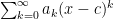, the most important thing is to determine the open interval of absolute convergence; that is, the intervals on which converges.

We teach that these intervals are *always* symmetric about (that is, at only, on some open interval or the whole real line. Side note: this is an interesting place to point out the influence that the calculus of complex variables has on real variable calculus! These open intervals are the most important aspect as one can prove that one can differentiate and integrate said series “term by term” on the open interval of absolute convergence; sometimes one can extend the results to the boundary of the interval.

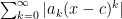
Therefore, if time is limited, I tend to focus on material more relevant for series that are absolutely convergent though there are some interesting (and fun) things one can do for a series which is conditionally convergent (convergent, but not absolutely convergent; e. g. .

Important principles: I think it is a good idea to first deal with geometric series and then series with positive terms…make that “non-negative” terms.

Geometric series: ; here we see that for , and is equal to for ; to show this do the old “shifted sum” addition: , then subtract: as most of the terms cancel with the subtraction.

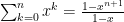
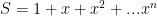
Now to show the geometric series converges, (convergence being the standard kind: the “n’th partial sum, then the series converges if an only if the sequence of partial sums converges; yes there are other types of convergence)

Now that we’ve established that for the geometric series, and we get convergence if goes to zero, which happens only if .

Why geometric series: two of the most common series tests (root and ratio tests) involve a comparison to a geometric series. Also, the geometric series concept is used both in the theory of improper integrals and in measure theory (e. g., showing that the rational numbers have measure zero).

Series of non-negative terms. For now, we’ll assume that has all (suppressing the indices).

Main principle: though most texts talk about the various tests, I believe that most of the tests involved really involve three key principles, two of which the geometric series and the following result from sequences of positive numbers:

Key sequence result: every monotone bounded sequence of positive numbers converges to its least upper bound.

True: many calculus texts don’t do that much with the least upper bound concept but I feel it is intuitive enough to at least mention. If the least upper bound is, say, , then if is the sequence in question, there has to be some such that for any small, positive . Then because is monotone, for all

The third key principle is “common sense” : if converges (standard convergence) then as a sequence. This is pretty clear if the are non-negative; the idea is that the sequence of partial sums cannot converge to a limit unless becomes arbitrarily small. Of course, this is true even if the terms are not all positive.

Secondary results I think that the next results are “second order” results: the main results depend on these, and these depend on the key 3 that we just discussed.

The first of these secondary results is the direct comparison test for series of non-negative terms:

Direct comparison test

If and converges, then so does . If diverges, then so does .

The proof is basically the “bounded monotone sequence” principle applied to the partial sums. I like to call it “if you are taller than an NBA center then you are tall” principle.

Evidently, some see this result as a “just get to something else” result, but it is extremely useful; one can apply this to show that the exponential of a square matrix is defined; it is the principle behind the Weierstrass M-test, etc. Do not underestimate this test!

Absolute convergence: this is the most important kind of convergence for power series as this is the type of convergence we will have on an open interval. A series is absolutely convergent if converges. Now, of course, absolute convergence implies convergence:

Note and if converges, then converges by direct comparison. Now note is the difference of two convergent series: and therefore converges.

Integral test This is an important test for convergence at a point. This test assumes that is a non-negative, non-decreasing function on some (that is, ) Then converges if and only if converges as an improper integral.

Proof: is just a right endpoint Riemann sum for and therefore the sequence of partial sums is an increasing, bounded sequence. Now if the sum converges, note that is the right endpoint estimate for so the integral can be defined as a limit of a bounded, increasing sequence so the integral converges.

Yes, these are crude whiteboards but they get the job done.

Note: we need the hypothesis that is decreasing (or non-decreasing). Example: the function certainly has converging but diverging.

Going the other way, defining gives an unbounded function with unbounded sum but the integral converges to the sum . The “boxes” get taller and skinnier.

Note: the above shows the integral and sum starting at 0; same principle though.

Now wait a minute: we haven’t really gone over how students will do most of their homework and exam problems. We’ve covered none of these: p-test, limit comparison test, ratio test, root test. Ok, logically, we have but not practically.

Let’s remedy that. First, start with the “point convergence” tests.

p-test. This says that converges if and diverges otherwise. Proof: Integral test.

Limit comparison test Given two series of positive terms: and

Suppose

If converges and then so does .

If diverges and then so does

I’ll show the “converge” part of the proof: choose then such that This means and we get convergence by direct comparison. See how useful that test is?

But note what is going on: it really isn’t necessary for to exist; for the convergence case it is only necessary that there be some for which ; if one is familiar with the limit superior (“limsup”) that is enough to make the test work.

We will see this again.

Why limit comparison is used: Something like clearly converges, but nailing down the proof with direct comparison can be hard. But a limit comparison with is pretty easy.

Ratio test this test is most commonly used when the series has powers and/or factorials in it. Basically: given consider (if the limit exists..if it doesn’t..stay tuned).

If the series converges. If the series diverges. If the test is inconclusive.

Note: if it turns out that there is exists some such that for all we have then the series converges (we can use the limsup concept here as well)

Why this works: suppose there exists some such that for all we have Then write

now factor out a to obtain

Now multiply the terms by 1 in a clever way:

See where this is going: each ratio is less than so we have:

which is a convergent geometric series.

See: there is geometric series and the direct comparison test, again.

Root Test No, this is NOT the same as the ratio test. In fact, it is a bit “stronger” than the ratio test in that the root test will work for anything the ratio test works for, but there are some series that the root test works for that the ratio test comes up empty.

I’ll state the “lim sup” version of the ratio test: if there exists some such that, for all we have then the series converges (exercise: find the “divergence version”).

As before: if the condition is met, so the original series converges by direction comparison.

Now as far as my previous remark about the ratio test: Consider the series:

Yes, this series is bounded by the convergent geometric series with and therefore converges by direct comparison. And the limsup version of the root test works as well.

But the ratio test is a disaster as which is unbounded..but .

What about non-absolute convergence (aka “conditional convergence”)

Series like converges but does NOT converge absolutely (p-test). On one hand, such series are a LOT of fun..but the convergence is very slow and unstable and so might say that these series are not as important as the series that converges absolutely. But there is a lot of interesting mathematics to be had here.

So, let’s chat about these a bit.

We say is conditionally convergent if the series converges but diverges.

One elementary tool for dealing with these is the alternating series test:

for this, let and for all .

Then converges if and only if as a sequence.

That the sequence of terms goes to zero is necessary. That it is sufficient in this alternating case: first note that the terms of the sequence of partial sums are bounded above by (as the magnitudes get steadily smaller) and below by (same reason. Note also that so the sequence of partial sums of even index are an increasing bounded sequence and therefore converges to some limit, say, . But and so by a routine “epsilon-N” argument the odd partial sums converge to as well.

Of course, there are conditionally convergent series that are NOT alternating. And conditionally convergent series have some interesting properties.

One of the most interesting properties is that such series can be “rearranged” (“derangment” in Knopp’s book) to either converge to any number of choice or to diverge to infinity or to have no limit at all.

Here is an outline of the arguments:

To rearrange a series to converge to , start with the positive terms (which must diverge as the series is conditionally convergent) and add them up to exceed ; stop just after is exceeded. Call that partial sum . Note: this could be 0 terms. Now use the negative terms to go of the left of and stop the first one past. Call that Then move to the right, past again with the positive terms..note that the overshoot is smaller as the terms are smaller. This is . Then go back again to get to the left of . Repeat.

Note that at every stage, every partial sum after the first one past is between some and the bracket and the distance is shrinking to become arbitrarily small.

To rearrange a series to diverge to infinity: Add the positive terms to exceed 1. Add a negative term. Then add the terms to exceed 2. Add a negative term. Repeat this for each positive integer .

Have fun with this; you can have the partial sums end up all over the place.

That’s it for now; I might do power series later.

Series convergence tests: the “harder to use in calculus 1” tests may well be the most useful.

I talked about the root and ratio test here and how the root test is the stronger of the two tests. What I should point out that the proof of the root test depends on the basic comparison test.

And so..a professor on Twitter asked:

https://twitter.com/MathProfPeter/status/1385606921156284429

Of course, one proves the limit comparison test by the direct comparison test. But in a calculus course, the limit comparison test might appear to be more readily useful..example:

Show converges.

So..what about the direct comparison test?

As someone pointed out: the direct comparison can work very well when you don’t know much about the matrix.

One example can be found when one shows that the matrix exponential where is a matrix.

For those unfamiliar: where the powers make sense as is square and we merely add the corresponding matrix entries.

What enables convergence is the factorial in the denominators of the individual terms; the i-j’th element of each can get only so large.

But how does one prove convergence?

The usual way is to dive into matrix norms; one that works well is (just sum up the absolute value of the elements (the Taxi cab norm or norm )

Then one can show and and together this implies the following:

For any index where is the i-j’th element of we have:

It then follows that . Therefore every series that determines an entry of the matrix is an absolutely convergent series by direct comparison. and is therefore a convergent series.

More fun with selective sums of divergent series

Just a reminder: if is a series and is some sequence consisting of 0’s and 1’s then a selective sum of the series is . The selective sum concept is discussed in the MAA book Real Infinite Series (MAA Textbooks) by Bonar and Khoury (2006) and I was introduced to the concept by Ferdinands’s article Selective Sums of an Infinite Series in the June 2015 edition of Mathematics Magazine (Vol. 88, 179-185).

There is much of interest there, especially if one considers convergent series or alternating series.

This post will be about divergent series of positive terms for which and for all .

The first fun result is this one: any selected is a selective sum of such a series. The proof of this isn’t that bad. Since we can find a smallest such that . Clearly if we are done: our selective sum has and the rest of the .

If not, set and note that because the series diverges, there is a largest so that . Now if we are done, else let and note . Now because the tend to zero, there is some first so that . If this is equality then the required sum is , else we can find the largest so that

This procedure can be continued indefinitely. So if we label we see that form an increasing, bounded sequence which converges to the least upper bound of its range, and it isn’t hard to see that the least upper bound is because

So now that we can obtain any positive real number as the selective sum of such a series, what can we say about the set of all selective sums for which almost all of the (that is, all but a finite number of the are zero).

Answer: the set of all such selective sums are dense in the real line, and this isn’t that hard to see, given our above construction. Let be any open interval in the real line and let . Then one can find some such that for all we have . Now consider our construction and choose large enough such that . Then the represents the finite selected sum that lies in the interval .

We can be even more specific if we now look at a specific series, such as the harmonic series . We know that the set of finite selected sums forms a dense subset of the real line. But it turns out that the set of select sums is the rationals. I’ll give a slightly different proof than one finds in Bonar and Khoury.

First we prove that every rational in is a finite select sum. Clearly 1 is a finite select sum. Otherwise: Given we can find the minimum so that . If we are done. Otherwise: the strict inequality shows that which means . Then note and this fraction has a strictly smaller numerator than . So we can repeat our process with this new rational number. And this process must eventually terminate because the numerators generated from this process form a strictly decreasing sequence of positive integers. The process can only terminate when the new faction has a numerator of 1. Hence the original fraction is some sum of fractions with numerator 1.

Now if the rational number in question is greater than one, one finds so that but . Then write and note that its magnitude is less than . We then use the procedure for numbers in noting that our starting point excludes the previously used terms of the harmonic series.

There is more we can do, but I’ll stop here for now.

More Fun with Divergent Series: redefining series convergence (Cesàro, etc.)

This post is more designed to entertain myself than anything else. This builds up a previous post which talks about deleting enough terms from a divergent series to make it a convergent one.

This post is inspired by Chapter 8 of Konrad Knopp’s classic Theory and Application of Infinite Series. The title of the chapter is Divergent Series.

Notation: when I talk about a series converging, I mean “converging” in the usual sense; e. g. if and then is said to be convergent with sum .

All of this makes sense since things like limits are carefully defined. But as Knopp points out, in the “days of old”, mathematicians say these series as formal objects rather than the result of careful construction. So some of these mathematicians (like Euler) had no problem saying things like . Now this is complete nonsense by our usual modern definition. But we might note that for and note that IS in the domain of the left hand side.

So, is there a way of redefining the meaning of “infinite sum” that gives us this result, while not changing the value of convergent series (defined in the standard way)? As Knopp points out in his book, the answer is “yes” and he describes several definitions of summation that

1. Do not change the value of an infinite sum that converges in the traditional sense and
2. Allows for more series to coverge.

We’ll discuss one of these methods, commonly referred to as Cesàro summation. There are ways to generalize this.

How this came about

Consider the Euler example: . Clearly, and so this geometric series diverges. But notice that the arithmetic average of the partial sums, computed as does tend to as tends to infinity: whereas and both of these quantities tend to as tends to infinity.

So, we need to see that this method of summing is workable; that is, do infinite sums that converge in the previous sense still converge to the same number with this method?

The answer is, of course, yes. Here is how to see this: Let be a sequence that converges to zero. Then for any we can find such that implies that . So for we have Because is fixed, the first fraction tends to zero as tends to infinity. The second fraction is smaller than in absolute value. But is arbitrary, hence this arithmetic average of this null sequence is itself a null sequence.

Now let and let Now subtract note and the forms a null sequence. Then so do the .

Now to be useful, we’d have to show that series that are summable in the Cesàro obey things like the multiplicative laws; they do but I am too lazy to show that. See the Knopp book.

I will mention a couple of interesting (to me) things though. Neither is really profound.

1. If a series diverges to infinity (that is, if for any positive there exists such that for all , then this series is NOT Cesàro summable. It is relatively easy to see why: given such an then consider which is greater than for large . Hence the Cesàro partial sum becomes unbounded.

Upshot: there is no hope in making something like into a convergent series by this method. Now there is a way of making an alternating, divergent series into a convergent one via doing something like a “double Cesàro sum” (take arithmetic averages of the arithmetic averages) but that is a topic for another post.

2. Cesàro summation may speed up convergent of an alternating series which passes the alternating series test, OR it might slow it down. I’ll have to develop this idea more fully. But I invite the reader to try Cesàro summation for and on and on . In the first two cases, the series converges slowly enough so that Cesàro summation speeds up convergence. Cesàro slows down the convergence in the geometric series though. It is interesting to ponder why.

Trimming a divergent series into a convergent one

This post is motivated by this cartoon

which I found at a Evelyn Lamb’s post on an AMS Blog, this fun Forbes math post by Kevin Kundson and by a June 2015 article in Mathematics Magazine by R. John Ferdinands called Selective Sums of an Infinite Series.

Here is the following question: start with a divergent series of positive terms which form a decreasing (non-increasing) sequence which tends to zero, say, . Now how does one select a subset of series terms to delete so as to obtain a convergent series? The Kundson article shows that one can do this with the harmonic series by, say, deleting all numbers that contain a specific digit (say, 9). I’ll talk about the proof here. But I’d like to start more basic and to bring in language used in the Ferdinands article.

So, let’s set the stage: we will let denote the divergent sum in question. All terms will be positive, for all and . Now let represent a sequence where for all ; then is called a selective sum of . I’ll call the the selecting sequence and, from the start, rule out selecting sequences that are either eventually 1 (which means that the selected series diverges since the original series did) or eventually zero (just a finite sum).

Now we’ll state a really easy result:

There is some non-eventually constant such that converges. Here is why: because , for each one can find a maximal index so that . Now select if and otherwise. Then and therefore the selected series converges by comparison with a convergent geometric series.

Of course, this result is petty lame; this technique discards a lot of terms. A cheap way to discard “fewer” terms (“fewer” meaning: in terms of “set inclusion”): Do the previous construction, but instead of using use where is a positive integer of choice. Note that

Here is an example of how this works: Consider the divergent series and the convergent geometric series Of course so but then for we have . So for . But because . The next non-zero selection coefficient is as .

Now playing with this example, we see that for but not for . So for and . So the first few are . Of course the gap between the grows as does.

Now let’s get back to the cartoon example. From this example, we’ll attempt to state a more general result.

Claim: given where if contains a 9 as one of its digits, then converges. Hint on how to prove this (without reading the solution): count the number of integers between and that lack a 9 as a digit. Then do a comparison test with a convergent geometric series, noting that every term is less than or equal to .

How to prove the claim: we can start by “counting” the number of integers between 0 and that contain no 9’s as a digit.

Between 0 and 9: clearly 0-8 inclusive, or 9 numbers.

Between 10 and 99: a moment’s thought shows that we have numbers with no 9 as a digit (hint: consider 10-19, 20-29…80-89) so this means that we have numbers between 0 and 99 with no 9 as a digit.

This leads to the conjecture: there are numbers between 0 and with no 9 as a digit and between and with no 9 as a digit.

This is verified by induction. This is true for

Assume true for . Then to find the number of numbers without a 9 between and we get which then means we have numbers between 0 and with no 9 as a digit. So our conjecture is proved by induction.

Now note that

This establishes that

So it follows that and hence our selected sum is convergent.

Further questions: ok, what is going on is that we threw out enough terms of the harmonic series for the series to converge. Between terms and we allowed terms to survive.

This suggests that if we permit up to terms between and to survive ( fixed and positive) then we will have a convergent series. I’d be interested in seeing if there is an generalization of this.

But I am tried, I have a research article to review and I need to start class preparation for the upcoming spring semester. So I’ll stop here. For now. 🙂

Cantor sets and countable products of discrete spaces (0, 1)^Z

This might seem like a strange topic but right now our topology class is studying compact metric spaces. One of the more famous of these is the “Cantor set” or “Cantor space”. I discussed the basics of these here.

Now if you know the relationship between a countable product of two point discrete spaces (in the product topology) and Cantor spaces/Cantor Sets, this post is probably too elementary for you.

Construction: start with a two point set and give it the discrete topology. The reason for choosing 0 and 2 to represent the elements will become clear later. Of course, is a compact metric space (with the discrete metric: if .

Now consider the infinite product of such spaces with the product topology: where each is homeomorphic to . It follows from the Tychonoff Theorem that is compact, though we can prove this directly: Let be any open cover for . Then choose an arbitrary from this open cover; because we are using the product topology where each is a one or two point set. This means that the cardinality of is at most which requires at most elements of the open cover to cover.

Now let’s examine some properties.

Clearly the space is Hausdorff ( ) and uncountable.

1. Every point of is a limit point of . To see this: denote by the sequence where . Then any open set containing is and contains ALL points where for . So all points of are accumulation points of ; in fact they are condensation points (or perfect limit points ).

(refresher: accumulation points are those for which every open neighborhood contains an infinite number of points of the set in question; condensation points contain an uncountable number of points, and perfect limit points are those for which every open neighborhood contains as many points as the set in question has (same cardinality).

2. is totally disconnected (the components are one point sets). Here is how we will show this: given there exists disjoint open sets . Proof of claim: if there exists a first coordinate for which (that is, a first for which the canonical projection maps disagree ( ). Then
,

are the required disjoint open sets whose union is all of .

3. is countable, as basis elements for open sets consist of finite sequences of 0’s and 2’s followed by an infinite product of .

4. is metrizable as well; . Note that is metric is well defined. Suppose . Then there is a first . Then note

which is impossible.

5. By construction is uncountable, though this follows from the fact that is compact, Haudorff and dense in itself.

6. is homeomorphic to . The homeomorphism is given by . It follows that is homeomorphic to a finite product with itself (product topology). Here we use the fact that if is a continuous bijection with compact and Hausdorff then is a homeomorphism.

Now we can say a bit more: if is a copy of then is homeomorphic to . This will follow from subsequent work, but we can prove this right now, provided we review some basic facts about countable products and counting.

First lets show that there is a bijection between and . A bijection is suggested by this diagram:

which has the following formula (coming up with it is fun; it uses the fact that :

for even
for odd
for odd,
for even,

Here is a different bijection; it is a fun exercise to come up with the relevant formulas:

Now lets give the map between and . Let and denote the elements of by where .

We now describe a map by

Example:

That this is a bijection between compact Hausdorff spaces is immediate. If we show that is continuous, we will have shown that is a homeomorphism.

But that isn’t hard to do. Let be open; . Then there is some for which . Then if denotes the component of we wee that for all (these are entries on or below the diagonal containing depending on whether is even or odd.

So is of the form where each is open in . This is an open set in the product topology of so this shows that is continuous. Therefore is a homeomorphism, therefore so is .

Ok, what does this have to do with Cantor Sets and Cantor Spaces?

If you know what the “middle thirds” Cantor Set is I urge you stop reading now and prove that that Cantor set is indeed homeomorphic to as we have described it. I’ll give this quote from Willard, page 121 (Hardback edition), section 17.9 in Chapter 6:

The proof is left as an exercise. You should do it if you think you can’t, since it will teach you a lot about product spaces.

What I will do I’ll give a geometric description of a Cantor set and show that this description, which easily includes the “deleted interval” Cantor sets that are used in analysis courses, is homeomorphic to .

Set up
I’ll call this set and describe it as follows:

(for those interested in the topology of manifolds this poses no restrictions since any manifold embeds in for sufficiently high ).

Reminder: the diameter of a set will be
Let be a strictly decreasing sequence of positive real numbers such that .

Let be some closed n-ball in (that is, is a subset homeomorphic to a closed n-ball; we will use that convention throughout)

Let be two disjoint closed n-balls in the interior of , each of which has diameter less than .

Let be disjoint closed n-balls in the interior and be disjoint closed n-balls in the interior of , each of which (all 4 balls) have diameter less that . Let

To describe the construction inductively we will use a bit of notation: for all and will represent an infinite sequence of such .
Now if has been defined, we let and be disjoint closed n-balls of diameter less than which lie in the interior of . Note that consists of disjoint closed n-balls.

Now let . Since these are compact sets with the finite intersection property ( for all ), is non empty and compact. Now for any choice of sequence we have is nonempty by the finite intersection property. On the other hand, if then so choose such that . Then lie in different components of since the diameters of these components are less than .

Then we can say that the uniquely define the points of . We can call such points

Note: in the subspace topology, the are open sets, as well as being closed.

Finding a homeomorphism from to .
Let be defined by . This is a bijection. To show continuity: consider the open set . Under this pulls back to the open set (in the subspace topology) hence is continuous. Because is compact and is Hausdorff, is a homeomorphism.

This ends part I.

We have shown that the Cantor sets defined geometrically and defined via “deleted intervals” are homeomorphic to . What we have not shown is the following:

Let be a compact Hausdorff space which is dense in itself (every point is a limit point) and totally disconnected (components are one point sets). Then is homeomorphic to . That will be part II.

Compact spaces and Tychonoff’s Theorem I

Note to the reader: when I first started this post, I thought it would be a few easy paragraphs. The size began to swell, so I am taking this post in several bite sized parts. This is part I.

Pretty much everyone knows what a compact space is. But not everyone is up on equivalent definitions and on how to prove that the arbitrary product of compact spaces is compact.
The genesis of this blog post is David Wright’s Proceedings of the American Mathematical Society paper (1994) on Tychonoff’s Theorem.

Since I am also writing for my undergraduate topology class, I’ll keep things elementary where possible and perhaps put in more detail than a professional mathematician would have patience for.

I should start by saying why this topic is dear to me: my research area is knot theory; in particular I studied embeddings of the circle into the 3-dimensional sphere , which can be thought of as the “compactification” of ; basically one starts with and then adds a point and declares that the neighborhoods of this new point will be generated by sets of the following form: The reason we do this: we often study the complement of the embedded circle, and it is desirable to have a compact set as the complement.

I’ve also studied (in detail) certain classes of embeddings of the real line into non-compact manifolds; to make this study a bit more focused, I insist that such embeddings be “proper” in that the inverse image of a compact set be compact. Hence compactness comes up again, even when the objects of study are not compact.

So, what do we mean by “compact”?

Instead of just blurting out the definition and equivalent formulations, I’ll try to give some intuition. If we are talking about a subset of a metric space, a compact subset is one that is both closed and bounded. Now that is NOT the definition of compactness, though it is true that:

Given a set , is compact if and only if is both closed (as a topological subset) and bounded (in that it fits within a sufficiently large closed ball). In compact subsets can be thought of as selected finite unions and arbitrary intersections of closed intervals. In the higher dimensions, think of the finite union and arbitrary intersections of things like closed balls.

Now it is true that if is continuous, then if is a compact topological space, then is compact (either as a space, or in the subspace topology, if is not onto.

This leads to a big theorem of calculus: the Extreme Value Theorem: if is continuous over a compact subset then attains both a maximum and a minimum value over .

Now in calculus, we rarely use the word “compact” but instead say something about be a closed, bounded subset. In the case where we usually say that , a closed interval.

So, in terms of intuition, if one is thinking about subsets of , one can think of a compact space as a domain on which any continuous real valued function always attains both a minimum and a maximum value.

Now for the definition
We need some terminology: a collection of open sets is said to be an open cover of a space if and if a collection of open sets is said to be an open cover of if A finite subcover is a finite subcollection of the open sets such that .

Here is an example: is an open cover of in the subspace topology. A finite subcover (from this collection) would be

Let be a topological space. We say that is a compact topological space if any open over of has a finite subcover. If we say that is a compact subset of if any open cover of has a finite subcover.

Prior to going through examples, I think that it is wise to mention something. One logically equivalent definition is this: A space (or a subset) is compact if every cover by open basis elements has a finite subcover. Here is why: if is compact, then ANY open cover has a finite subcover, and an open cover by basis elements is an open cover. On the other hand: if we assume the “every open cover by open basis elements has a finite subcover” condition: then if is an open cover, then we can view this open cover as an open cover of the basis elements whose union is each open . This open cover of basis elements has a finite subcover of basis elements..say . Then for each basis element, choose a single for which . That is the required open subcover.

Now, when convenient, we can assume that the open cover in question (during a proof) consists of basic open sets. That will simplify things at times.

So, what are some compact spaces and sets, and what are some basic facts?

Let’s see some compact sets, some non compact sets and see some basic facts.

1. Let be any topological space and a finite subset. Then is a compact subset. Proof: given any open cover of choose one open set per element of which contains said element.

2. Let have the usual topology. Then the integers is not a compact subset; choose the open cover is an infinite cover with no finite subcover. In fact, ANY unbounded subset in the usual metric topology fails to be compact: for with choose ; clearly this open cover can have no finite subcover.

3. The finite union of compact subsets is compact (easy exercise).

4. If is compact and is a Hausdorff topological space () then is closed. Here is why: let and for every choose open where . Now is an open set which contains and has a finite subcover Note that each is an open set which contains and now we have only a finite number of these. Hence which is disjoint from which contains . Because was an arbitrary point in , is open which means that is closed. Note: this proof, with one minor addition, shows that a compact Hausdorff space is regular () we need only show that a closed subset of a compact Hausdorff space is compact. That is easy enough to do: let be an open cover for ; then the collection is an open cover for , which has a finite subcover. Let that be where each . Now since does not cover does.

So we have proved that a closed subset of a compact set is compact.

5. Let (or any infinite set) be given the finite complement topology (that is, the open sets are the empty set together with sets whose complements consist of a finite number of points). Then ANY subset is compact! Here is why: let be any set and let be any open cover. Choose . Since is a finite set of points, only a finite number of them can be in , say . Then for each of these, select one open set in the open cover that contains the point; that is the finite subcover.

Note: this shows that non-closed sets can be compact sets, if the underlying topology is not Hausdorff.

6. If is continuous and onto and is compact, then so is . Proof: let cover and note that covers , hence a finite number of these open sets cover: . Therefore covers . Note: this shows that being compact is a topological invariant; that is, if two spaces are homeomorphic, then either both spaces are compact or neither one is.

7. Ok, let’s finally prove something. Let have the usual topology. Then (and therefore any closed interval) is compact. This is (part) of the famous Heine-Borel Theorem. The proof uses the least upper bound axiom of the real numbers.

Let be any open cover for . If no finite subcover exists, let be the least upper bound of the subset of that CAN be covered by a finite subcollection of . Now because at least one element of contains and therefore contains for some . Assume that . Now suppose , that is is part of the subset that can be covered by a finite subcover. Then because for some then which means that , which means that isn’t an upper bound for .

Now suppose ; then because there is still some where . But since then and so . So if can be covered by then is a finite subcover of which means that was not an upper bound. It follows that which means that the unit interval is compact.

Now what about the closed ball in ? The traditional way is to show that the closed ball is a closed subset of a closed hypercube in and so if we show that the product of compact spaces is compact, we would be done. That is for later.

8. Now endow with the lower limit topology. That is, the open sets are generated by basis elements . Note that the lower limit topology is strictly finer than the usual topology. Now in this topology: is not compact. (note: none of are compact in the coarser usual topology, so there is no need to consider these). To see this, cover by and it is easy to see that this open cover has no finite subcover. In fact, with a bit of work, one can show that every compact subset is at most countable and nowhere dense; in fact, if is compact in the lower limit topology and there exists some where .

Power sets, Function spaces and puzzling notation

I’ll probably be posting point-set topology stuff due to my being excited about teaching the course…finally.

Power sets and exponent notation
If is a set, then the power set of , often denoted by , is a set that consists of all subsets of .

For example, if , then . Now is is no surprise that if the set is finite and has elements, then has elements.

However, there is another helpful way of listing . A subset of can be defined by which elements of that it has. So, if we order the elements of as then the power set of can be identified as follows:

So there is a natural correspondence between the elements of a power set and a sequence of binary digits. Of course, this makes the counting much easier.

The binary notation might seem like an unnecessary complication at first, but now consider the power set of the natural numbers: . Of course, listing the power sets would be, at least, cumbersome if not impossible! But there the binary notation really shows its value. Remember that the binary notation is a sequence of 0’s and 1’s where a 0 in the i’th slot means that element isn’t an element in a subset and a 1 means that it is.

Since a subset of the natural numbers is defined by its list of elements, every subset has an infinite binary sequence associated with it. We can order the sequence in the usual order 1, 2, 3, 4, ….
and the sequence 1, 0, 0, 0…… corresponds to the set with just 1 in it, the sequence 1, 0, 1, 0, 1, 0, 1, 0,… corresponds to the set consisting of all odd integers, etc.

Then, of course, one can use Cantor’s Diagonal Argument to show that is uncountable; in fact, if one uses the fact that every non-negative real number has a binary expansion (possibly infinite), one then shows that has the same cardinality as the real numbers.

Power notation
We can expand on this power notation. Remember that can be thought of setting up a “slot” or an “index” for each element of and then assigning a or for every element of . One can then think of this in an alternate way: can be thought of as the set of ALL functions from the elements of to the set . This coincides with the “power set” concept as set membership is determined by being either “in” or “not in”. So, the set in the exponent can be thought of either as the indexing set and the base as the value each indexed value can take on (sequences, in the case that the exponent set is either finite or countably finite), OR this can be thought of as the set of all functions where the exponent set is the domain and the base set is the range.

Remember, we are talking about ALL possible functions and not all “continuous” functions, or all “morphisms”, etc.

So, can be thought of as either set set of all possible sequences of positive integers, or, equivalently, the set of all functions of to .

Then is the set of all real number sequences (i. e. the types of sequences we study in calculus), or, equivalently, the set of all real valued functions of the positive integers.

Now it is awkward to try to assign an ordering to the reals, so when we consider it is best to think of this as the set of all functions , or equivalently, the set of all strings which are indexed by the real numbers and have real values.

Note that sequences don’t really seem to capture in the way that they capture, say, . But there is another concept that does, and that concept is the concept of the net, which I will talk about in a subsequent post.

Aitken acceleration: another “easy” example for the students

In a previous post I showed some spreadsheet data to demonstrate the Aitken acceleration process. Here, I’ll go through an example where a sequence converges linearly: let where . We use the form (I am too lazy to use the traditional “p-hat” notation). First, note that the denominator works out to

The numerator is a tiny bit more work: the terms cancel and as far as the rest:

which simplifies to a term involving and one that doesn’t. Here is the term involving :

which, of course, is just times the denominator.

Now the terms not involving :

So our fraction is merely

This can be rearranged to

Clearly as goes to infinity, the error goes to zero very quickly. It might be instructive to look at the ratio of the errors for and :

This ratio is

Note that in the right hand factor: both squared factors are fixed and the coefficients go to infinity as goes to infinity. If one multiplies out, one obtains:

. In the limit, the first term decreases to and the second goes to infinity.

Hence the errors in the accelerated sequence are smaller.

Demonstrating Aitken’s sequence acceleration

Right now, we are studying the various root finding algorithms in Numerical Analysis (bisection, Newton’s, etc.)

Such algorithms yield a sequence of numbers, which (hopefully) converge to a solution: .

Of course, each point in the sequence is obtained by calculations and, if there were a way to combine these points so as to obtain a sequence that converges faster (while not adding much to the computation complexity), there is some benefit. And yes, it is possible to use the sequence points, do the series manipulation and use the manipulated points in the root finding algorithm itself (e. g. Steffensen’s method).

In this post, I’ll talk about Aitken’s method and how one can cook up examples that not only show that the method can work but give the students some intuition as to why it might work.

I’ll provide just a bit of background in the event that the general reader comes across this.

Let . If we have ( is positive, of course) we say that the convergence is LINEAR if and the inequality must be strict. If then we say that convergence is quadratic (regardless of .)

To see the reason for the terminology, just multiply both sides of the “defining equation” by the denominator. In the linear case : so one can think: “get new approximation by multiplying the old approximation by some constant less than one”. For example: exhibits linear convergence to 0; that is a decent way to think about it.

Now (in the linear convergence case anyway), suppose you think of your approximation having an error that shrinks with iteration but shrinks in the following way: the n’th iteration looks like where are constants strictly between 0 and 1. Of course, as goes to infinity, approaches the limit as the error terms die away.

Aitken’s method is this: let’s denote a new sequence by . (I am not using the traditional P-hat out of laziness) Then . To see how this formula is obtained, check out these excellent course notes. Or the Wiki article is pretty good.

Look at the numerator of what is being subtracted off: if we have the terms written (very roughly) as and if, say, is much larger than , then will be closer to than is to , hence more of this error will be subtracted away.

Yes, I know that his is simple-minded, but it “gets the spirit” of the process. I’ve set up some spreadsheets with “cooked” sequences linearly converging to zero and showed how the Aitken process works there. Note: the spreadsheet round off errors start occurring at the range; you can see that here.

(click to see the larger image)

To see an abstract example where where , go to the next post in this series.