This always bothered me about partial fractions…

Let’s look at an “easy” starting example: write
We know how that goes: multiply both sides by to get and then since this must be true for ALL , substitute to get and then substitute to get . Easy-peasy.

BUT…why CAN you do such a substitution since the original domain excludes ?? (and no, I don’t want to hear about residues and “poles of order 1”; this is calculus 2. )

Lets start with with the restricted domain, say
Now multiply both sides by and note that, with the restricted domain we have:

But both sides are equal on the domain and the limit on the left hand side is So the right hand side has a limit which exists and is equal to . So the result follows..and this works for the calculation for B as well.

Yes, no engineer will care about this. But THIS is the reason we can substitute the non-domain points.

As an aside: if you are trying to solve something like one can do the denominator clearing, and, as appropriate substitute and compare real and imaginary parts ..and yes, now you can use poles and residues.

A tidbit with respect to Laplace transforms and sin(x)/x

I’ve discovered the channel “blackpenredpen” and it is delightful.
It is a nice escape into mathematics that, while far from research level, is “fun” and beyond mere fluff.

And that got me to thinking about . Yes, this can be done by residues

But I’ll look at this with Laplace Transforms.

We know that
But note that the antiderivative of with respect to is That might not seem like much help, but then notice (assuming

So why not:
Now since the left hand side is just a double integral over the first quadrant (an infinite rectangle) the order of integration can be interchanged:

and that is equal to .

Note: is sometimes called the function

\

How I am cutting corners in class

Ok, which is more difficult?

1. Solve using Laplace transforms or:

2. Given find the inverse Laplace transform.

Clearly, 2 is harder and in texts I’ve used, we had to do those prior to doing 1. But, in a way, you have to do 2 in order to do 1:

But this is already factored and students can be taught to “attempt to factor and if you can’t, complete the square” and this leads immediately to:

which can be resolved by partial fractions.

In our “one less week plus online” I will do much more of 1 than 2.

Of course, there is still some work to do; we still have to solve

I will teach the “eliminate the term method by using complex numbers:

Let to get

Let

So we have

The particular solution part pulls back to

There is a work to do for the other part:

To get the shift we have to add and subtract 3; this leads to:

(adjusting the second term for the
And this part pulls back to

Yeah, I know; if you are reading this, you already know this stuff, but I think using i helps speed things up a bit.

And yes, you could have just used the convolution integral and have been done with it, though one would have had to have used
and been done with it. (you remembered the 1/2, didn’t you? )

And my “clever proof” is dashed

It has been a while since I posted here, though I have been regularly posting in my complex variables class blog last semester.

And for those who like complex variables and numerical analysis, this is an exciting, interesting development.

A fundamental tension in numerical analysis is the interplay between truncation errors and rounding errors; this is particularly prevalent in the numerical approximation of #derivatives. @nhigham explores this concept in the current issue of #SIAMNews. https://t.co/QbNxAs44pN

— SIAM (@TheSIAMNews) June 6, 2018

But as to the title of my post: I was working to finish up a proof that one kind of wild knot is not “equivalent” to a different kind of wild knot and I had developed a proof (so I think) that the complement of one knot contains an infinite collection of inequivalent tori (whose solid tori contain the knot non-trivially) whereas the other kind of knot can only have a finite number of such tori. I still like the proof.

But it turns out that there is already an invariant that does the trick nicely..hence I can shorten and simplify the paper.

But dang it..I liked my (now irrelevant to my intended result) result!

And I trolled my complex variables class

One question on my last exam: find the Laurent series for centered at which converges on the punctured disk . And yes, about half the class missed it.

I am truly evil.

And I embarrass myself….integrate right over a couple of poles…

I didn’t have the best day Thursday; I was very sick (felt as if I had been in a boxing match..chills, aches, etc.) but was good to go on Friday (no cough, etc.)

So I walk into my complex variables class seriously under prepared for the lesson but decide to tackle the integral

Of course, you know the easy way to do this, right?

and evaluate the latter integral as follows:

(this follows from restricting to the unit circle and setting and then obtaining a rational function of which has isolated poles inside (and off of) the unit circle and then using the residue theorem to evaluate.

So And then the integral is transformed to:

Now the denominator factors: which means but only the roots lie inside the unit circle.
Let

Write:

Now calculate: and

Adding we get so by Cauchy’s theorem

Ok…that is fine as far as it goes and correct. But what stumped me: suppose I did not evaluate and divide by two but instead just went with:

$latex where is the upper half of ? Well, has a primitive away from those poles so isn’t this just , right?

So why not just integrate along the x-axis to obtain because the integrand is an odd function?

This drove me crazy. Until I realized…the poles….were…on…the…real…axis. ….my goodness, how stupid could I possibly be???

To the student who might not have followed my point: let be the upper half of the circle taken in the standard direction and if you do this property (hint: set . Now attempt to integrate from 1 to -1 along the real axis. What goes wrong? What goes wrong is exactly what I missed in the above example.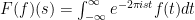

Posting went way down in 2017

I only posted 3 times in 2017. There are many reasons for this; one reason is the teaching load, the type of classes I was teaching, etc.

I spent some of the year creating a new course for the Business College; this is one that replaced the traditional “business calculus” class.

The downside: there is a lot of variation in that course; for example, one of my sections has 1/3 of the class having a math ACT score of under 20! And we have many who are one standard deviation higher than that.

But I am writing. Most of what I write this semester can be found at the class blog for our complex variables class.

Our class does not have analysis as a prerequisite so it is a challenge to make it a truly mathematical class while getting to the computationally useful stuff. I want the students to understand that this class is NOT merely “calculus with z instead of x” but I don’t want to blow them away with proofs that are too detailed for them.

The book I am using does a first pass at integration prior to getting to derivatives.

Fourier Transform of the “almost Gaussian” function with a residue integral

This is based on the lectures on the Fourier Transform by Brad Osgood from Stanford:

And here, provided the integral converges.

The “almost Gaussian” integrand is ; one can check that . One way is to use the fact that and do the substitution ; of course one should be able to demonstrate the fact to begin with. (side note: a non-standard way involving symmetries and volumes of revolution discovered by Alberto Delgado can be found here)

So, during this lecture, Osgood shows that ; that is, this modified Gaussian function is “its own Fourier transform”.

I’ll sketch out what he did in the lecture at the end of this post. But just for fun (and to make a point) I’ll give a method that uses an elementary residue integral.

Both methods start by using the definition:

Method 1: combine the exponential functions in the integrand:

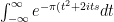. Now complete the square to get:

Now factor out the factor involving alone and write as a square:

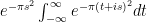
Now, make the substitution to obtain:

Now we show that the above integral is really equal to

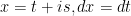
To show this, we perform along the retangular path 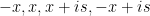: and let

Now the integral around the contour is 0 because is analytic.

We wish to calculate the negative of the integral along the top boundary of the contour. Integrating along the bottom gives 1.
As far as the sides: if we fix we note that and the magnitude goes to zero as So the integral along the vertical paths approaches zero, therefore the integrals along the top and bottom contours agree in the limit and the result follows.

Method 2: The method in the video
This uses “differentiation under the integral sign”, which we talk about here.

Stat with and note

Now we do integration by parts: and the integral becomes:

Now the first term is zero for all values of as . The second term is merely:

.

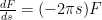So we have shown that which is a differential equation in which has solution (a simple separation of variables calculation will verify this). Now to solve for the constant note that .

The result follows.

Now: which method was easier? The second required differential equations and differentiating under the integral sign; the first required an easy residue integral.

By the way: the video comes from an engineering class. Engineers need to know this stuff!

Letting complex algebra make our calculus lives easier

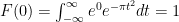If one wants to use complex arithmetic in elementary calculus, one should, of course, verify a few things first. One might talk about elementary complex arithmetic and about complex valued functions of a real variable at an elementary level; e. g. . Then one might discuss Euler’s formula: 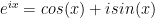and show that the usual laws of differentiation hold; i. e. show that and one might show that for an integer. The latter involves some dreary trigonometry but, by doing this ONCE at the outset, one is spared of having to repeat it later.

This is what I mean: suppose we encounter where is an even integer. I use an even integer power because is more challenging to evaluate when is even.

Coming up with the general formula can be left as an exercise in using the binomial theorem. But I’ll demonstrate what is going on when, say, .

So it follows reasonably easily that, for even,

So integration should be a breeze. Lets see about things like, say,

Of course these are known formulas, but their derivation is relatively simple when one uses complex expressions.

Where “j” comes from

I laughed at what was said from 30:30 to 31:05 or so:

If you are wondering why your engineering students want to use is is because, in electrical engineering, usually stands for “current”.

Though many of you know this, this lesson also gives an excellent reason to use the complex form of the Fourier series; e. g. if is piece wise smooth and has period 1, write (usual abuse of the equals sign) rather than writing it out in sines and cosines. of course, if is real valued.

How is this easier? Well, when you give a demonstration as to what the coefficients have to be (assuming that the series exists to begin with, the orthogonality condition is very easy to deal with. Calculate: for when . There is nothing to it; easy integral. Of course, one has to demonstrate the validity of and show that the usual differentiation rules work ahead of time, but you need to do that only once.