How I am cutting corners in class

Ok, which is more difficult?

1. Solve using Laplace transforms or:

2. Given find the inverse Laplace transform.

Clearly, 2 is harder and in texts I’ve used, we had to do those prior to doing 1. But, in a way, you have to do 2 in order to do 1:

But this is already factored and students can be taught to “attempt to factor and if you can’t, complete the square” and this leads immediately to:

which can be resolved by partial fractions.

In our “one less week plus online” I will do much more of 1 than 2.

Of course, there is still some work to do; we still have to solve

I will teach the “eliminate the term method by using complex numbers:

Let to get

Let

So we have

The particular solution part pulls back to

There is a work to do for the other part:

To get the shift we have to add and subtract 3; this leads to:

(adjusting the second term for the
And this part pulls back to

Yeah, I know; if you are reading this, you already know this stuff, but I think using i helps speed things up a bit.

And yes, you could have just used the convolution integral and have been done with it, though one would have had to have used
and been done with it. (you remembered the 1/2, didn’t you? )

A change of variable to determine if growth is still exponential

This video is pretty good, and I thought that I’d add some equations to the explanation:

So, in terms of the mathematics, what is going on?

The graph they came up with is “new confirmed cases” on the y-axis (log scale) and total number of cases on the x-axis. Let’s see what this looks like for exponential growth.

Here, letting the total number of cases at time be denoted by , the number of new cases is , the first derivative.

In the case of exponential growth, where is positive.

which is what is being plotted on the y-axis. So with the change of variable we are letting and our new function is , which, of course, is a straight line through the origin. That is, of course, IF the growth is exponential.

To get a feel for what this looks like, suppose we had polynomial growth; say . Then In the case of linear growth we’d have (constant) and for, say, , or a “concave down” function.

Now for the logistic situation in which the number of cases grows exponentially at first and then starts to level out to some steady state value, call it , the relationship between the number of cases and the new number of cases looks like so our which is a quadratic which opens down.

Yes, this gets studied in differential equations class when we study autonomous differential equations.

Now for some graphs:

This is exponential growth vs. logistic growth; we get something similar to the latter when cases start to peak.

Here, I tweaked the logistic model to have the same derivative as the exponential model near .

Here: we have linear growth vs the

Here: cubic growth vs.

My review lessons online

We had an extra week to prepare to teach online, so I put notes from the previous few weeks up in blog form:

Blog

Blog

Blog

That was quite a bit of work, but I did find some cool videos out there and embedded them in my lessons.

My teaching during the COVID-19 Pandemic

My university has moved to “online only” for the rest of the semester. I realize that most of us are in the same boat.
Fortunately, for now, I’ve got some academic freedom to make changes and I am taking a different approach than some.

Some appear to be wanting to keep things “as normal as possible.”

For me: the pandemic changes everything.

Yes, there are those on the beach in Florida. That isn’t most of my students; it could be some of them.

So, here is what will be different for me:
1) I am making exams “open book, open note” and take home: they get it and are given several days to do it and turn it back in, like a project.
Why? Fluid situations, living with a family, etc. might make it difficult to say “you HAVE to take it now…during period X.” This is NOT an online class that they signed up for.
Yes, it is possible that some cheat; that can’t be helped.

Also, studying will be difficult to do. So, getting a relatively long “designed as a programmed text” is, well, getting them to study WHILE DOING THE EXAM. No, it is not the same as “study to put it in your brain and then show you know it” at exam time. But I feel that this gets them to learn while under this stressful situation; they take time aside to look up and think about the material. The exam, in a way, is going through a test bank.

2) Previously, I thought of testing as serving two purposes: a) it encourages students to review and learn and b) distinguishing those with more knowledge from those with lesser knowledge. Now: tests are to get the students to learn..of course diligence will be rewarded. But who does well and who does not..those groups might change a little.

3) Quiz credit: I was able to sign up for webassign, and their quizzes will be “extra credit” to build on their existing grade. This is a “carrot only” approach.

4) Most of the lesson delivery will be a polished set of typeset notes with videos. My classes will be a combination of “live chat” with video where I will discuss said notes and give tips on how to do problems. I’ll have office hours ..some combination of zoom meetings which people can join and I’ll use e-mail to set up “off hours” meetings, either via chat or zoom, or even an exchange of e-mails.

We shall see how it works; I have a plan and think I can execute it, but I make no guarantee of the results.
Yes, there are polished online classes, but those are designed to be done deliberately. What we have here is something made up at the last minute for students who did NOT sign up for it and are living in an emergency situation.

Over-scheduling of senior faculty and lower division courses: how important is course prep?

It seems as if the time faculty is expected to spend on administrative tasks is growing exponentially. In our case: we’ve had some administrative upheaval with the new people coming in to “clean things up”, thereby launching new task forces, creating more committees, etc. And this is a time suck; often more senior faculty more or less go through the motions when it comes to course preparation for the elementary courses (say: the calculus sequence, or elementary differential equations).

And so:

1. Does this harm the course quality and if so..
2. Is there any effect on the students?

I should first explain why I am thinking about this; I’ll give some specific examples from my department.

1. Some time ago, a faculty member gave a seminar in which he gave an “elementary” proof of why is non-elementary. Ok, this proof took 40-50 minutes to get through. But at the end, the professor giving the seminar exclaimed: “isn’t this lovely?” at which, another senior member (one who didn’t have a Ph. D. had had been around since the 1960’s) asked “why are you happy that yet again, we haven’t had success?” The fact that a proof that could not be expressed in terms of the usual functions by the standard field operations had been given; the whole point had eluded him. And remember, this person was in our calculus teaching line up.

2. Another time, in a less formal setting, I had mentioned that I had given a brief mention to my class that one could compute and improper integral (over the real line) of an unbounded function that that a function could have a Laplace transform. A junior faculty member who had just taught differential equations tried to inform me that only functions of exponential order could have a Laplace transform; I replied that, while many texts restricted Laplace transforms to such functions, that was not mathematically necessary (though it is a reasonable restriction for an applied first course). (briefly: imagine a function whose graph consisted of a spike of height at integer points over an interval of width and was zero elsewhere.

3. In still another case, I was talking about errors in answer keys and how, when I taught courses that I wasn’t qualified to teach (e. g. actuarial science course), it was tough for me to confidently determine when the answer key was wrong. A senior, still active research faculty member said that he found errors in an answer key..that in some cases..the interval of absolute convergence for some power series was given as a closed interval.

I was a bit taken aback; I gently reminded him that was such a series.

I know what he was confused by; there is a theorem that says that if converges (either conditionally or absolutely) for some then the series converges absolutely for all where The proof isn’t hard; note that convergence of means eventually, for some positive then compare the “tail end” of the series: use and then and compare to a convergent geometric series. Mind you, he was teaching series at the time..and yes, is a senior, research active faculty member with years and years of experience; he mentored me so many years ago.

4. Also…one time, a sharp young faculty member asked around “are there any real functions that are differentiable exactly at one point? (yes: try if is rational, if is irrational.

5. And yes, one time I had forgotten that a function could be differentiable but not be (try: at

What is the point of all of this? Even smart, active mathematicians forget stuff if they haven’t reviewed it in a while…even elementary stuff. We need time to review our courses! But…does this actually affect the students? I am almost sure that at non-elite universities such as ours, the answer is “probably not in any way that can be measured.”

Think about it. Imagine the following statements in a differential equations course:

1. “Laplace transforms exist only for functions of exponential order (false)”.
2. “We will restrict our study of Laplace transforms to functions of exponential order.”
3. “We will restrict our study of Laplace transforms to functions of exponential order but this is not mathematically necessary.”

Would students really recognize the difference between these three statements?

Yes, making these statements, with confidence, requires quite a bit of difference in preparation time. And our deans and administrators might not see any value to allowing for such preparation time as it doesn’t show up in measures of performance.

Numerical solutions to differential equations: I wish that I had heard this talk first

The MAA Mathfest in Chicago was a success for me. I talked about some other talks I went to; my favorite was probably the one given by Douglas Arnold. I wish I had had this talk prior to teaching numerical analysis for the fist time.

Confession: my research specialty is knot theory (a subset of 3-manifold topology); all of my graduate program classes have been in pure mathematics. I last took numerical analysis as an undergraduate in 1980 and as a “part time, not taking things seriously” masters student in 1981 (at UTSA of all places).

In each course…I. Made. A. “C”.

Needless to say, I didn’t learn a damned thing, even though both professors gave decent courses. The fault was mine.

But…I was what my department had, and away I went to teach the course. The first couple of times, I studied hard and stayed maybe 2 weeks ahead of the class.
Nevertheless, I found the material fascinating.

When it came to understanding how to find a numerical approximation to an ordinary differential equation (say, first order), you have: with some initial value for both . All of the techniques use some sort of “linearization of the function” technique to: given a step size, approximate the value of the function at the end of the next step. One chooses a step size, and some sort of schemes to approximate an “average slope” (e. g. Runga-Kutta is one of the best known).

This is a lot like numerical integration, but in integration, one knows for all values; here you have to infer from previous approximations of %latex y(t) $. And there are things like error (often calculated by using some sort of approximation to such as, say, the Taylor polynomial, and error terms which are based on things like the second derivative.

And yes, I faithfully taught all that. But what was unknown to me is WHY one might choose one method over another..and much of this is based on the type of problem that one is attempting to solve.

And this is the idea: take something like the Euler method, where one estimates . You repeat this process a bunch of times thereby obtaining a sequence of approximations for . Hopefully, you get something close to the “true solution” (unknown to you) (and yes, the Euler method is fine for existence theorems and for teaching, but it is too crude for most applications).

But the Euler method DOES yield a piecewise linear approximation to SOME which might be close to (a good approximation) or possibly far away from it (a bad approximation). And this that you actually get from the Euler (or other method) is important.

It turns out that some implicit methods (using an approximation to obtain and then using THAT to refine your approximation can lead to a more stable system of (the solution that you actually obtain…not the one that you are seeking to obtain) in that this system of “actual functions” might not have a source or a sink…and therefore never spiral out of control. But this comes from the mathematics of the type of equations that you are seeking to obtain an approximation for. This type of example was presented in the talk that I went to.

In other words, we need a large toolbox of approximations to use because some methods work better with certain types of problems.

I wish that I had known that before…but I know it now. 🙂

Trolled by Newton’s Law of Cooling…

From a humor website: there is a Facebook account called “customer service” who trolls customers making complaints. Though that isn’t a topic here, it is interesting to see Newton’s Cooling Law get mentioned:

One upside to a topologist teaching numerical analysis…

Yes, I was glad when we hired people with applied mathematics expertise; though I am enjoying teaching numerical analysis, it is killing me. My training is in pure mathematics (in particular, topology) and so class preparation is very intense for me.

But I so love being able to show the students the very real benefits that come from the theory.

Here is but one example: right now, I am talking about numerical solutions to “stiff” differential equations; basically, a differential equation is “stiff” if the magnitude of the differential equation is several orders of magnitude larger than the magnitude of the solution.

A typical example is the differential equation , for . Example: . Note that the solution decays very quickly to zero though the differential equation is 20 times larger.

One uses such an equation to test a method to see if it works well for stiff differential equations. One such method is the Euler method: which becomes . There is a way of assigning a method to a polynomial; in this case the polynomial is and if the roots of this polynomial have modulus less than 1, then the method will converge. Well here, the root is and calculating: which implies that . This is a good reference.

So for we find that has to be less than . And so I ran Euler’s method for the initial problem on and showed that the solution diverged wildly for using 9 intervals, oscillated back and forth (with equal magnitudes) for using 10 intervals, and slowly converged for using 11 intervals. It is just plain fun to see the theory in action.

Osgood’s uniqueness theorem for differential equations

I am teaching a numerical analysis class this semester and we just started the section on differential equations. I want them to understand when we can expect to have a solution and when a solution satisfying a given initial condition is going to be unique.

We had gone over the “existence” theorem, which basically says: given and initial condition where where is some rectangle in the plane, if is a continuous function over , then we are guaranteed to have at least one solution to the differential equation which is guaranteed to be valid so long as stays in .

I might post a proof of this theorem later; however an outline of how a proof goes will be useful here. With no loss of generality, assume that and the rectangle has the lines as vertical boundaries. Let , the line of slope . Now partition the interval into and create a polygonal path as follows: use slope at , slope at and so on to the right; reverse this process going left. The idea: we are using Euler’s differential equation approximation method to obtain an initial piecewise approximation. Then do this again for step size

In this way, we obtain an infinite family of continuous approximation curves. Because is continuous over , it is also bounded, hence the curves have slopes whose magnitude are bounded by some . Hence this family is equicontinuous (for any given one can use in continuity arguments, no matter which curve in the family we are talking about. Of course, these curves are uniformly bounded, hence by the Arzela-Ascoli Theorem (not difficult) we can extract a subsequence of these curves which converges to a limit function.

Seeing that this limit function satisfies the differential equation isn’t that hard; if one chooses close enough, one shows that where then the differential equation has exactly one solution where which is valid so long as the graph remains in .

Here is the proof: where . This is clear but perhaps a strange step.
But now suppose that there are two solutions, say and where . So set and note the following: and . A Mean Value Theorem argument applied to means that we can assume that we can select our so that on that interval (since ).

So, on this selected interval about we have (we can remove the absolute value signs.).

Now we set up the differential equation: which has a unique solution whose graph is always positive; . Note that the graphs of meet at . But where .

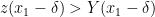But since on that interval.

So, no such point can exist.

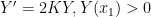Note that we used the fact that the solution to is always positive. Though this is an easy differential equation to solve, note the key fact that if we tried to separate the variables, we’d calculate and find that this is an improper integral which diverges to positive hence its primitive cannot change sign nor reach zero. So, if we had where is an infinite improper integral and , we would get exactly the same result for exactly the same reason.

Hence we can recover Osgood’s Uniqueness Theorem which states:

If is continuous on and for all we have a where where is a positive function and diverges to at then the differential equation has exactly one solution where which is valid so long as the graph remains in .

Ok, what do you see here? (why we don’t blindly trust software)

I had Dfield8 from MATLAB propose solutions to meeting the following initial conditions:

.

Now, of course, one of these solutions is non-unique. But, of all of the solutions drawn: do you trust ANY of them? Why or why not?

Note: you really don’t have to do much calculus to see what is wrong with at least one of these. But, if you must know, the general solution is given by (and, of course, the equilibrium solution ). But that really doesn’t provide more information that the differential equation does.

By the way, here are some “correct” plots of the solutions, (up to uniqueness)