I was in a weird situation this semester in my “applied calculus” (aka “business calculus”) class. I had an awkward amount of time left (1 week) and I still wanted to do something with Taylor polynomials, but I had nowhere near enough time to cover infinite series and power series.
So, I just went ahead and introduced it “user’s manual” style, knowing that I could justify this, if I had to (and no, I didn’t), even without series. BUT there are some drawbacks too.
Let’s see how this goes. We’ll work with series centered at (expand about 0) and assume that has as many continuous derivatives as desired on an interval connecting 0 to .
Now we calculate: , of course. But we could do the integral another way: let’s use parts and say . Note the choice for and that is a constant in the integral. We then get . Evaluation:
and we’ve completed the first step.
Though we *could* do the inductive step now, it is useful to grind through a second iteration to see the pattern.
We take our expression and compute by parts again, with and insert into our previous expression:
which works out to:
and note the alternating sign of the integral.
Now to use induction: assume that:
Now let’s look at the integral: as usual, use parts as before and we obtain:
. Taking some care with the signs we end up with
which works out to .
Substituting this evaluation into our inductive step equation gives the desired result.
And note: NOTHING was a assumed except for having the required number of continuous derivatives!
BUT…yes, there is a catch. The integral is often regarded as a “correction term.” But the Taylor polynomial is really only useful so long as the integral can be made small. And that is the issue with this approach: there are times when the integral cannot be made small; it is possible that can be far enough out that the associated power series does NOT converge on and the integral picks that up, but it may well be hidden, or at least non-obvious.
And that is why, in my opinion, it is better to do series first.
Let’s show an example.
Consider . We know from work with the geometric series that its series expansion is and that the interval of convergence is But note that is smooth over and so our Taylor polynomial, with integral correction, should work for .
So, nothing that our k-th Taylor polynomial relation is:
Let’s focus on the integral; the “remainder”, if you will.
Rewrite it as: .
Now this integral really isn’t that hard to do, if we use an algebraic trick:
Rewrite
Now the integral is a simple substitutions integral: let so our integral is transformed into:
This remainder cannot be made small if no matter how big we make
But, in all honesty, this remainder could have been computed with simple algebra.
and now solve for algebraically .
The larger point is that the “error” is hidden in the integral remainder term, and this can be tough to see in the case where the associated Taylor series has a finite radius of convergence but is continuous on the whole real line, or a half line.
This is “part 2” of a previous post about series. Once again, this is not designed for students seeing the material for the first time.
I’ll deal with general power series first, then later discuss Taylor Series (one method of obtaining a power series).
General Power Series Unless otherwise stated, we will be dealing with series such as though, of course, a series can expanded about any point in the real line (e. g. ) Note: unless it is needed, I’ll be suppressing the index in the summation sign.
So, IF we have a function ..
what do we mean by this and what can we say about it?
The first thing to consider, of course, is convergence. One main fact is that the open interval of convergence of a power series centered at 0 is either: 1. Non existent …series converges at only (e. g. ; try the ratio test) or
2. Converges absolutely on for some and diverges for all (like a geometric series) (anything possible for ) or
3. Converges absolutely on the whole real line.
Many texts state this result but do not prove it. I can understand as this result is really an artifact of calculus of a complex variable. But it won’t hurt to sketch out a proof at least for the “converge” case for so I’ll do that.
So, let’s assume that converges (either absolute OR conditional ) So, by the divergence test, we know that the sequence of terms . So we can find some index such that
So write: and converges absolutely for . The divergence follows from a simple “reversal of the inequalities (that is, if the series diverged at ).
Though the relation between real and complex variables might not be apparent, it CAN be useful. Here is an example: suppose one wants to find the open interval of convergence of, say, the series representation for ? Of course, the function itself is continuous on the whole real line. But to find the open interval of convergence, look for the complex root of that is closest to zero. That would be so the interval is
So, what about a function defined as a power series?
For one, a power series expansion of a function at a specific point (say, ) is unique:
Say on the interval of convergence, then substituting yields . So subtract from both sides and get: . Now assuming one can “factor out an x” from both sides (and you can) we get , etc.
Yes, this should have property been phrased as a limit and I’ve yet to show that is continuous on its open interval of absolute convergence.
Now if you say “doesn’t that follow from uniform convergence which follows from the Weierstrass M test” you’d be correct…and you are probably wasting your time reading this.
Now if you remember hearing those words but could use a refresher, here goes:
We want for sufficiently close AND both within the open interval of absolute convergence, say Choose where and such that and where (these are just polynomials).
The rest follows:
Calculus On the open interval of absolute convergence, a power series can be integrated term by term and differentiated term by term. Neither result, IMHO, is “obvious.” In fact, sans extra criteria, for series of functions, in general, it is false. Quickly: if you remember Fourier Series, think about the Fourier series for a rectangular pulse wave; note that the derivative is zero everywhere except for the jump points (where it is undefined), then differentiate the constituent functions and get a colossal mess.
Differentiation: most texts avoid the direct proof (with good reason; it is a mess) but it can follow from analysis results IF one first shows that the absolute (and uniform) convergence of implies the absolute (and uniform) convergence of
So, let’s start here: if is absolutely convergent on then so is .
Here is why: because we are on the open interval of absolute convergence, WLOG, assume and find where is also absolutely convergent. Now, note that so the series converges by direct comparison on which establishes what we wanted to show.
Of course, this doesn’t prove that the expected series IS the derivative; we have a bit more work to do.
Again, working on the open interval of absolute convergence, let’s look at:
Now, we use the fact that is absolutely convergent on and given any we can find so that for between and
So let’s do that: pick and then note:
Now apply the Mean Value Theorem to each term in the second term:
where each is between and . By the choice of the second term is less than , which is arbitrary, and the first term is the first terms of the “expected” derivative series.
So, THAT is “term by term” differentiation…and notice that we’ve used our hypothesis …almost all of it.
Term by term integration
Theoretically, integration combines easier with infinite summation than differentiation does. But given we’ve done differentiation, we can then do anti-differentiation by showing that converges and then differentiating.
But let’s do this independently; it is good for us. And we’ll focus on the definite integral.
(of course, )
Once again, choose so that
Then and this is less than (or equal to)
But is arbitrary and so the result follows, for definite integrals. It is an easy exercise in the Fundamental Theorem of Calculus to extract term by term anti-differentiation.
Taylor Series
Ok, now that we can say stuff about a function presented as a power series, what about finding a power series representation for a function, PROVIDED there is one? Note: we’ll need the function to have an infinite number of derivatives on an open interval about the point of expansion. We’ll also need another condition, which we will explain as we go along.
We will work with expanding about . Let be the function of interest and assume all of the relevant derivatives exist.
Start with which can be thought of as our “degree 0” expansion plus remainder term.
But now, let’s use integration by parts on the integral with (it is a clever choice for ; it just has to work.
So now we have:
It looks like we might run into sign trouble on the next iteration, but we won’t as we will see: do integration by parts again:
and so we have:
This turns out to be .
An induction argument yields
For the series to exist (and be valid over an open interval) all of the derivatives have to exist and;
.
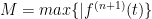
Note: to get the Lagrange remainder formula that you see in some texts, let for and then
It is a bit trickier to get the equality as the error formula; it is a Mean Value Theorem for integrals calculation.
About the remainder term going to zero: this is necessary. Consider the classic counterexample:
It is an exercise in the limit definition and L’Hopital’s Rule to show that for all and so a Taylor expansion at zero is just the zero function, and this is valid at 0 only.
As you can see, the function appears to flatten out near x =0 $ but it really is NOT constant.
Note: of course, using the Taylor method isn’t always the best way. For example, if we were to try to get the Taylor expansion of at it is easier to use the geometric series for and substitute ; the uniqueness of the power series expansion allows for that.
Of course, one proves the limit comparison test by the direct comparison test. But in a calculus course, the limit comparison test might appear to be more readily useful..example:
Show converges.
So..what about the direct comparison test?
As someone pointed out: the direct comparison can work very well when you don’t know much about the matrix.
One example can be found when one shows that the matrix exponential where is a matrix.
For those unfamiliar: where the powers make sense as is square and we merely add the corresponding matrix entries.
What enables convergence is the factorial in the denominators of the individual terms; the i-j’th element of each can get only so large.
But how does one prove convergence?
The usual way is to dive into matrix norms; one that works well is (just sum up the absolute value of the elements (the Taxi cab norm or norm )
Then one can show and and together this implies the following:
For any index where is the i-j’th element of we have:
It then follows that . Therefore every series that determines an entry of the matrix is an absolutely convergent series by direct comparison. and is therefore a convergent series.
Chebyshev (or Tchebycheff) polynomials are a class of mutually orthogonal polynomials (with respect to the inner product: ) defined on the interval . Yes, I realize that this is an improper integral, but it does converge in our setting.
These are used in approximation theory; here are a couple of uses:
1. The roots of the Chebyshev polynomial can be used to find the values of that minimize the maximum of over the interval . This is important in minimizing the error of the Lagrange interpolation polynomial.
2. The Chebyshev polynomial can be used to adjust an approximating Taylor polynomial to increase its accuracy (away from the center of expansion) without increasing its degree.
Let’s discuss the polynomials themselves. They are defined for all positive integers as follows:
. Now, it is an interesting exercise in trig identities to discover that these ARE polynomials to begin with; one shows this to be true for, say, by using angle addition formulas and the standard calculus resolution of things like . Then one discovers a relation: to calculate the rest.
The definition allows for some properties to be calculated with ease: the zeros occur when and the first derivative has zeros where ; these ALL correspond to either an endpoint max/min at or local max and mins whose values are also . Here are the graphs of
Now here is a key observation: the graph of a forms spanning arcs in the square and separates the square into regions. So, if there is some other function whose graph is a connected, piecewise smooth arc that is transverse to the graph of that both spans the square from to and that stays within the square, that graph must have points of intersection with the graph of .
Now suppose that is the graph of a polynomial of degree whose leading coefficient is and whose graph stays completely in the square . Then the polynomial has degree (because the leading terms cancel via the subtraction) but has roots (the places where the graphs cross). That is clearly impossible; hence the only such polynomial is .
This result is usually stated in the following way: is normalized to be monic (have leading coefficient 1) by dividing the polynomial by and then it is pointed out that the normalized is the unique monic polynomial over that stays within for all . All other monic polynomials have a graph that leaves that box at some point over .
Of course, one can easily cook up analytic functions which don’t leave the box but these are not monic polynomials of degree .
Ok, you say, “this works”; this is a series representation for . Ok, it is but why?
Now if you tell me: and that and term by term integration yields: I’d remind you of: “interval of absolute convergence” and remind you that the series for does NOT converge at and that one has to be in the open interval of convergence to justify term by term integration.
True, the series DOES converge to but it is NOT that elementary to see. 🙂
One of the many good things about my teaching career is that as I teach across the curriculum, I fill in the gaps of my own education.
I got my Ph. D. in topology (low dimensional manifolds; in particular, knot theory) and hadn’t seen much of differential equations beyond my “engineering oriented” undergraduate course.
Therefore, I learned more about existence and uniqueness theorems when I taught differential equations; though I never taught the existence and uniqueness theorems in a class, I learned the proofs just for my own background. In doing so I learned about the Picard iterated integral technique for the first time; how this is used to establish “uniqueness of solution” can be found here.
However I recently discovered (for myself) what thousands of mathematicians already know: the Picard process can be used to yield an interval of existence for a solution for a differential equation, even if we cannot obtain the solution in closed form.
The situation
I assigned my numerical methods class to solve with and to produce the graph of from to .
There is a unique solution to this and the solution is valid so long as the and value of the solution curve stays finite; note that
So, is it possible that the values for this solution become unbounded?
Answer: yes. What follows are the notes I gave to my class.
Numeric output seems to indicate this, but numeric output is NOT proof.
To find a proof of this, let’s turn to the Picard iteration technique. We
know that the Picard iterates will converge to the unique solution.
The integrals get pretty ugly around here; I used MATLAB to calculate the
higher order iterates. I’ll show you
where means assorted polynomial terms from order 6 to 11.
Here is one more:
We notice some patterns developing here. First of all, the coefficient of
the term is staying the same for all where
That is tedious to prove. But what is easier to show (and sufficient) is
that the coefficients for the terms for all appear to be
bigger than 1. This is important!
Why? If we can show that this is the case, then our ”limit” solution will have an interval of convergence less than 1. Why? Substitute and see that the sum
diverges because the not only fail to converge to zero, but they
stay greater than 1.
So, can we prove this general pattern?
YES!
Here is the idea: where is a polynomial of order
and is a polynomial whose terms all have order or greater.
Now put into the Picard process:
Note: all of the terms of of degree or higher must come from
the second integral.
Now by induction we can assume that all of the coefficients of the
polynomial are greater than or equal to one.
When we ”square out” the polynomial, the coefficients of the new
polynomial will consist of the sum of positive numbers, each of which is
greater than 1. For the coefficients of the polynomial of
degree or higher: if one is interested in the
coefficient, one has to add at least numbers together, each of which
is bigger than one.
Now when one does the integration on these particular terms, one, of course,
divides by (power rule for integration). But that means that the
coefficient (after integration) is then greater than 1.
Here is a specific example:
Say
Now
Remember that are all greater than or equal to one.
Now
Now when we integrate term by term, we get:
But note that and
Since all of the factors are greater than or equal to 1.
Hence in our new polynomial approximation, the order 4 terms or less all
have coefficients which are greater than or equal to one.
We can make this into a Proposition:
Proposition
Suppose where each
If
Then for all
Proof. Of course, and
Let
Then we can calculate: (since all of the are
defined):
If is odd, then
If is even then
The Proposition is proved.
Of course, this possibly fails for where as we would fail to
have a sufficient number of terms in our sum.
Now if one wants a challenge, one can modify the above arguments to show that the coefficients of the approximating polynomial never get ”too big”; that is, the coefficient of the order term is less than, say, .
It isn’t hard to show that where
Then one can compare to the derivative of the geometric series to show that
one gets convergence on an interval up to but not including 1.
I am going to take a break from the Lebesgue stuff and maybe write more on that tomorrow.
My numerical analysis class just turned in some homework and some really have some misunderstanding about Taylor Series and Power Series. I’ll provide some helpful hints to perplexed students.
For the experts who might be reading this: my assumption is that we are dealing with functions which are real analytic over some interval. To students: this means that can be differentiated as often as we’d like, that the series converges absolutely on some open interval and that the remainder term goes to zero as the number of terms approaches infinity.
This post will be about computing such a series.
First, I’ll give a helpful reminder that is crucial in calculating these series: a Taylor series is really just a power series representation of a function. And if one finds a power series which represents a function over a given interval and is expanded about a given point, THAT SERIES IS UNIQUE, no matter how you come up with it. I’ll explain with an example:
Say you want to represent over the interval . You could compute it this way: you probably learned about the geometric series and that for .
Well, you could compute it by Taylor’s theorem which says that such a series can be obtained by: If you do such a calculation for one obtains , , and plugging into Taylor’s formula leads to the usual geometric series. That is, the series can be calculated by any valid method; one does NOT need to retreat to the Taylor definition for calculation purposes.
Example: in the homework problem, students were asked to calculate Taylor polynomials (of various orders and about ) for a function that looked like this:
. Some students tried to calculate the various derivatives and plug into Taylor’s formula with grim results. It is much easier than that if one remembers that power series are unique! Sure, one CAN use Taylor’s formula but that doesn’t mean that one should. Instead it is much easier if one remembers that Now to get one just substitutes for and obtains: . Then and one subtracts off to obtain the full power series:
Now calculating the bound for the remainder after terms is, in general, a pain. Sure, one can estimate with a graph, but that sort of defeats the point of approximating to begin with; one can use thumb rules which overstate the magnitude of the remainder term.


 though, of course, a series can expanded about any point in the real line (e. g.
  ) Note: unless it is needed, I’ll be suppressing the index in the summation sign.
 ..
.. only (e. g.
  ; try the ratio test) or
  for some
  and diverges for all
  (like a geometric series) (anything possible for
  ) or
) or converges (either absolute OR conditional ) So, by the divergence test, we know that the sequence of terms
  . So we can find some index
  such that
 and
and  converges absolutely for
  . The divergence follows from a simple “reversal of the inequalities (that is, if the series diverged at
  ).
). ? Of course, the function itself is continuous on the whole real line. But to find the open interval of convergence, look for the complex root of
  that is closest to zero. That would be
  so the interval is
 ) is unique:
 on the interval of convergence, then substituting
  yields
  . So subtract from both sides and get:
  . Now assuming one can “factor out an x” from both sides (and you can) we get
  , etc.
  is continuous on its open interval of absolute convergence.
 for
for  sufficiently close AND both within the open interval of absolute convergence, say
  where
where  and
and  and
and  where
where  (these are just polynomials).


 then so is
  .
. where
where  is also absolutely convergent. Now, note that
  so the series
  converges by direct comparison on
 is absolutely convergent on
  we can find
  so that
  for
for  between
 and then note:


 where each
  is between
  the second term is less than
  , which is arbitrary, and the first term is the first
  terms of the “expected” derivative series.
 converges and then differentiating.
  (of course,
 ![[a,b] \subset (-r, r)](https://s0.wp.com/latex.php?latex=%5Ba%2Cb%5D+%5Csubset+%28-r%2C+r%29+&bg=ffffff&fg=000000&s=0&c=20201002) )
)
 and this is less than (or equal to)
 be the function of interest and assume all of the relevant derivatives exist.
  which can be thought of as our “degree 0” expansion plus remainder term.
  (it is a clever choice for
  ; it just has to work.
 and so we have:
 .
.
 .
. for
for ![t \in [0,x]](https://s0.wp.com/latex.php?latex=t+%5Cin+%5B0%2Cx%5D+&bg=ffffff&fg=000000&s=0&c=20201002) and then
and then 
 as the error formula; it is a Mean Value Theorem for integrals calculation.
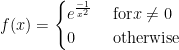
 for all
  and so a Taylor expansion at zero is just the zero function, and this is valid at 0 only.
 at
at  and substitute
  ; the uniqueness of the power series expansion allows for that.
  converges.
  where
where  is a
is a  matrix.
  where the powers make sense as
  is square and we merely add the corresponding matrix entries.
  can get only so large.
 (just sum up the absolute value of the elements (the Taxi cab norm or
  norm )
  and
and  and together this implies the following:
 is the i-j’th element of
![| [ e^A ]_{i,j} | \leq \sum^{\infty}_{k=0} {|A^k |\over k!} \leq \sum^{\infty}_{k=0} {|A|^k \over k!} =e^{|A|}](https://s0.wp.com/latex.php?latex=%7C+%5B+e%5EA+%5D_%7Bi%2Cj%7D+%7C+%5Cleq+%5Csum%5E%7B%5Cinfty%7D_%7Bk%3D0%7D+%7B%7CA%5Ek+%7C%5Cover+k%21%7D+%5Cleq++%5Csum%5E%7B%5Cinfty%7D_%7Bk%3D0%7D+%7B%7CA%7C%5Ek+%5Cover+k%21%7D+%3De%5E%7B%7CA%7C%7D+&bg=ffffff&fg=000000&s=0&c=20201002) . Therefore every series that determines an entry of the matrix
. Therefore every series that determines an entry of the matrix  ) defined on the interval
 ![[-1, 1]](https://s0.wp.com/latex.php?latex=%5B-1%2C+1%5D+&bg=ffffff&fg=000000&s=0&c=20201002) . Yes, I realize that this is an improper integral, but it does converge in our setting.
. Yes, I realize that this is an improper integral, but it does converge in our setting.![x_0, x_1, x_2, ...x_k \in [-1,1]](https://s0.wp.com/latex.php?latex=x_0%2C+x_1%2C+x_2%2C+...x_k+%5Cin+%5B-1%2C1%5D+&bg=ffffff&fg=000000&s=0&c=20201002) that minimize the maximum of
that minimize the maximum of  over the interval
 ![[-1,1]](https://s0.wp.com/latex.php?latex=%5B-1%2C1%5D+&bg=ffffff&fg=000000&s=0&c=20201002) . This is important in minimizing the error of the
. This is important in minimizing the error of the  to increase its accuracy (away from the center of expansion) without increasing its degree.
 . Now, it is an interesting exercise in trig identities to discover that these ARE polynomials to begin with; one shows this to be true for, say,
  by using angle addition formulas and the standard calculus resolution of things like
  . Then one discovers a relation:
  to calculate the rest.
  definition allows for some properties to be calculated with ease: the zeros occur when
  and the first derivative has zeros where
  ; these ALL correspond to either an endpoint max/min at
  or local max and mins whose
  values are also
  . Here are the graphs of


 forms
forms ![[-1, 1] \times [-1,1]](https://s0.wp.com/latex.php?latex=%5B-1%2C+1%5D+%5Ctimes+%5B-1%2C1%5D+&bg=ffffff&fg=000000&s=0&c=20201002) and separates the square into
and separates the square into  regions. So, if there is some other function
  to
to  and that stays within the square, that graph must have
  and whose graph stays completely in the square
  has degree
  (because the leading terms cancel via the subtraction) but has
  .
. is normalized to be monic (have leading coefficient 1) by dividing the polynomial by
 ![[-\frac{1}{2^{n-1}}, \frac{1}{2^{n-1}}]](https://s0.wp.com/latex.php?latex=%5B-%5Cfrac%7B1%7D%7B2%5E%7Bn-1%7D%7D%2C+%5Cfrac%7B1%7D%7B2%5E%7Bn-1%7D%7D%5D&bg=ffffff&fg=000000&s=0&c=20201002) for all
for all ![x \in [-1,1]](https://s0.wp.com/latex.php?latex=x+%5Cin+%5B-1%2C1%5D+&bg=ffffff&fg=000000&s=0&c=20201002) . All other monic polynomials have a graph that leaves that box at some point over
. All other monic polynomials have a graph that leaves that box at some point over 
 . Ok, it is but why?
 and that
  and term by term integration yields:
 I’d remind you of: “interval of absolute convergence” and remind you that the series for
  does NOT converge at
  but it is NOT that elementary to see. 🙂
 with
with  and to produce the graph of
  from
from  to
to  .
. and
and  value of the solution curve stays finite; note that


 means assorted polynomial terms from order 6 to 11.
 term is staying the same for all
  where
where 
 all appear to be
 will have an interval of convergence less than 1. Why? Substitute
  and see that the sum
 not only fail to converge to zero, but they
 where
where  is a polynomial of order
 is a polynomial whose terms all have order
  or greater.

 of degree
  or higher must come from
 are greater than or equal to one.
 of
of or higher: if one is interested in the
 numbers together, each of which
 (power rule for integration). But that means that the

 are all greater than or equal to one.

 and
and 
 where each


 and
and 

 are
are

 where
where  as we would fail to
 order term is less than, say,
  .
.  where
where 
 over the interval
  for
for  .
. If you do such a calculation for
  one obtains
  ,
,  ,
,  and plugging into Taylor’s formula leads to the usual geometric series. That is, the series can be calculated by any valid method; one does NOT need to retreat to the Taylor definition for calculation purposes.
 . Some students tried to calculate the various derivatives and plug into Taylor’s formula with grim results. It is much easier than that if one remembers that power series are unique! Sure, one CAN use Taylor’s formula but that doesn’t mean that one should. Instead it is much easier if one remembers that
  Now to get
  one just substitutes
  for
for  . Then
  and one subtracts off
  to obtain the full power series:
