This post is intended to help the student who is willing to put time and effort into succeeding in a college calculus class.
Part One: How to Study
The first thing to remember is that most students will have to study outside of class in order to learn the material. There are those who pick things up right away, but these students tend to be the rare exception.
Think of it this way: suppose you want to learn to play the piano. A teacher can help show you how to play it and provide a practice schedule. But you won’t be any good if you don’t practice.
Suppose you want to run a marathon. A coach can help you with running form, provide workout schedules and provide feedback. But if you don’t run those workouts, you won’t build up the necessary speed and endurance for success.
The same principle applies for college mathematics classes; you really learn the material when you study it and do the homework exercises.
Here are some specific tips on how to study:
1. It is optimal if you can spend a few minutes scanning the text for the upcoming lesson. If you do this, you’ll be alert for the new concepts as they are presented and the concepts might sink in quicker.
2. There is some research that indicates:
a. It is better to have several shorter study sessions rather than one long one and
b. There is an optimal time delay between study sessions and the associated lecture.
Look at it this way: if you wait too long after the lesson to study it, you would have forgotten much of what was presented. If you study right away, then you really have, in essence, a longer class room session. It is probably best to hit the material right when the initial memory starts to fade; this time interval will vary from individual to individual. For more on this and for more on learning for long term recall, see this article.
3. Learn the basic derivative formulas inside and out; that is, know what the derivatives of functions like  are on sight; you shouldn’t have to think about them. The same goes for the basic trig identities such as
  and
and 
Why is this? The reason is that much of calculus (though not all!) boils down to pattern recognition.
For example, suppose you need to calculate:

If you don’t know your differentiation formulas, this problem is all but impossible. On the other hand, if you do know your differentiation formulas, then you’ll immediately recognize the  and it’s derivative
  and you’ll see that this problem is really the very easy problem
  .
.
But this all starts with having “automatic” knowledge of the derivative formulas.
Note: this learning is something your professor or TA cannot do for you!
4. Be sure to do some study problems with your notes and your book closed. If you keep flipping to your notes and book to do the homework problems, you won’t be ready for the exams. You have to kick up the training wheels.
Try this; the difference will surprise you. There is also evidence that forcing yourself to recall the material FROM YOUR OWN BRAIN helps you learn the material! Give yourself frequent quizzes on what you are learning.
5. When reviewing for an exam, study the problems in mixed fashion. For example, get some note cards and write problems from the various sections on them (say, some from 3.1, some from 3.2, some from 3.3, and so on), mix the cards, then try the problems. If you just review section by section, you’ll go into each problem knowing what technique to use each time right from the start. Many times, half of the battle is knowing which technique to use with each problem; that is part of the course! Do the problems in mixed order.
If you find yourself whining complaining “I don’t know where to start” it means that you don’t know the material well enough. Remember that a trained monkey can repeat specific actions; you have to be a bit better than that!
6. Read the book, S L O W L Y, with pen and paper nearby. Make sure that you work through the examples in the text and that you understand the reasons for each step.
7. For the “more theoretical” topics, know some specific examples for specific theorems. Here is what I am talking about:
a. Intermediate value theorem: recall that if  , then
  but there is no
  such that
  . Why does this not violate the intermediate value theorem?
b. Mean value theorem: note also that there is no  such that
  . Why does this NOT violate the Mean Value Theorem?
c. Series: it is useful to know basic series such as those for  . It is also good to know some basic examples such as the geometric series, the divergent harmonic series
  and the conditionally convergent series
  .
.
d. Limit definition of derivative: be able to work a few basic examples of the derivative via the limit definition:  and know why the derivative of
  and
and  do not exist at
  .
.
Having some “template” example can help you master a theoretical concept.
Part II: Attitude
Your attitude will be very important.
1. Remember that your effort will be essential! Again, you can’t learn to run a marathon without getting off of the couch and making your muscles sore. Learning mathematics involves some frustration and, yes, at times, some tedium. Learning is fun OVERALL but it isn’t always fun at all times. You will encounter discomfort and unpleasantness at times.
2. Remember that winners look for ways to succeed; losers and whiners look for excuses for failure. You can always find those who will be willing to enable your underachievement. Instead, seek out those who bring out your best.
3. Success is NOT guaranteed; that is what makes success rewarding! Think of how good you’ll feel about yourself if you mastered something that seemed impossible to master at first. And yes, anyone who has achieved anything that is remotely difficult has taken some lumps and bruises along the way. You will NOT be spared these.
Remember that if you duck the calculus challenge, you are, in essence, slamming many doors of opportunity shut right from the get-go.
4. On the other hand, remember that Calculus (the first two semesters anyway) is a Freshman level class; exceptional mathematical talent is not a prerequisite for success. True, calculus is easy for some but that isn’t the point. Most reasonably intelligent people can have success, if they are willing to put forth the proper effort in the proper manner.
Just think of how good it will feel to succeed in an area that isn’t your strong suit!


![x \in (0,1]](https://s0.wp.com/latex.php?latex=x+%5Cin+%280%2C1%5D+&bg=ffffff&fg=000000&s=0&c=20201002)


![x \in [\frac{-1}{2}, \frac{1}{2}]](https://s0.wp.com/latex.php?latex=x+%5Cin+%5B%5Cfrac%7B-1%7D%7B2%7D%2C+%5Cfrac%7B1%7D%7B2%7D%5D+&bg=ffffff&fg=000000&s=0&c=20201002)


![f(x-t)f(t)=\left\{\begin{array}{c} 1,x \in [-1,0], -\frac{1}{2} t \le \frac{1}{2}+x \\ 1 ,x\in [0,1], -\frac{1}{2}+x \le t \le \frac{1}{2} \\ 0 \text{ elsewhere} \end{array}\right.](https://s0.wp.com/latex.php?latex=f%28x-t%29f%28t%29%3D%5Cleft%5C%7B%5Cbegin%7Barray%7D%7Bc%7D+1%2Cx+%5Cin+%5B-1%2C0%5D%2C+-%5Cfrac%7B1%7D%7B2%7D+t+%5Cle+%5Cfrac%7B1%7D%7B2%7D%2Bx+%5C%5C+1+%2Cx%5Cin+%5B0%2C1%5D%2C+-%5Cfrac%7B1%7D%7B2%7D%2Bx+%5Cle+t+%5Cle+%5Cfrac%7B1%7D%7B2%7D+%5C%5C+0+%5Ctext%7B+elsewhere%7D+%5Cend%7Barray%7D%5Cright.++&bg=ffffff&fg=000000&s=0&c=20201002)


![x \in [0,1]](https://s0.wp.com/latex.php?latex=x+%5Cin+%5B0%2C1%5D+&bg=ffffff&fg=000000&s=0&c=20201002)

 where
where 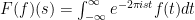 provided the integral converges.
  ; one can check that
  . One way is to use the fact that
  and do the substitution
  ; of course one should be able to
  ; that is, this modified Gaussian function is “its own Fourier transform”.
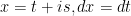
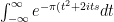 . Now complete the square to get:
 alone and write as a square:
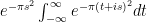
 to obtain:

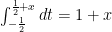
 along the retangular path
  :
: 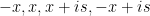 and let

 is analytic.
  and the magnitude goes to zero as
 and the integral becomes:
 . The second term is merely:
 .
.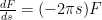 which is a differential equation in
  (a simple separation of variables calculation will verify this). Now to solve for the constant
  note that
 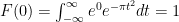 .
. 

 represent the tent map: the support of
  is
is ![[-1,1]](https://s0.wp.com/latex.php?latex=%5B-1%2C1%5D+&bg=ffffff&fg=000000&s=0&c=20201002) and it has the following graph:
and it has the following graph:![f(x)=\left\{\begin{array}{c} x+1,x \in [-1,0) \\ 1-x ,x\in [0,1] \\ 0 \text{ elsewhere} \end{array}\right.](https://s0.wp.com/latex.php?latex=f%28x%29%3D%5Cleft%5C%7B%5Cbegin%7Barray%7D%7Bc%7D+x%2B1%2Cx+%5Cin+%5B-1%2C0%29+%5C%5C+1-x+%2Cx%5Cin+%5B0%2C1%5D+%5C%5C+0+%5Ctext%7B+elsewhere%7D+%5Cend%7Barray%7D%5Cright.++&bg=ffffff&fg=000000&s=0&c=20201002)

 and do the integrals:
 and substitute and simplify later:
 and the next two have the same anti-derivative which can be obtained by a “integration by parts” calculation:
  ; evaluating the limits yields:
 . NOW use
  and we have the integral is
  by Euler’s formula.
 so
so  so our answer is
  which is often denoted as
  as
as  function
 (as we want the function to have zeros at integers and to “equal” one at
  made the algebra a whole lot easier.
 describes the heat in a one dimensional circle of metal and the radius is one, one can do the analysis of the heat equation
  with initial condition
  and assuming that
  has a Fourier expansion (complex coefficients) one can obtain:
  which can be rewritten as
  . Note:
  ranges from
  to
to  and by
  we mean
  and note that
  are complex conjugates for all
  . Now let
  then we could say that
  which is a convolution product;
  is the heat kernel which is a nice form. But about that interchange: when can we do it?
  we mean the limit of the sequence of partial sums:
  and if
  then the interchange is valid. NOTE: I am following the custom of not using the “differential”
  and of letting it be understood that
  means
means  .
.  are all measurable functions and
  (pointwise) and there exists an integrable function
  where
where  for all
  , then
  .
. .
.  , there are conditions that must be met to get that the the
  which means that
  exists. The mathematics of convergence of a Fourier series is rich; for this note we will assume that the Fourier series in question converges.
 then
then  but we need to use the Lebesgue integral to guarantee this equality..in general. This is why:
  and define
  and then inductively define
  . Then
  and for each
  ,
,  but
but  uniformly if for any
  there exists
  such that for all
  ,
,  for ALL
  in the interval of interest. Then, it a routine exercise in Riemann integration to see that if
  . The down side is that we rarely have uniform convergence when we are talking about Fourier series terms. Here is why: it is known that if