My research

If you are interested, I’ll be posting on topics that deal with my current area of research here.

I am reproducing this post below but will NOT publish further installments on this blog:

A knot is an embedding of the circle into 3-space. By “3-space” we usually mean or , which is the 3-sphere, which can be thought of as with a point added at infinity. is sometimes preferred because it is a compact space.

Note: sometimes we focus on the image of the embedding itself (i. e., the geometric object) and sometimes we focus on the map, which includes information about orientation.

Example: If one has then is a knot. Here are two different MATLAB plots of the image:

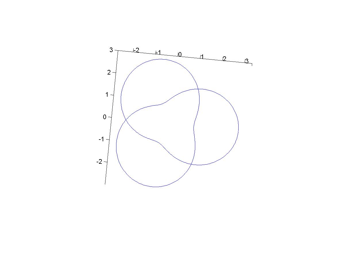
The second is a projection of the image of the trefoil onto the plane. If we endow such a projection with “crossing information”, we call the image a diagram for the knot.

Here, the broken line indicates that the strand passes under another strand.

It is custom to insist on “regular” projections, which means that:

1. All “singularities” (points on the diagram which correspond to more than one point of the knot) are double points (there are no points where 3 or more strands of the knot’s projection meet)
2. All crossings are “honest” crossings; that is there are no “tangents” (places where the projection “kisses” another strand).

Note: one can think of a diagram as a “shadow” of the knot on a plane, provided one adds crossing information at all double points.

Now not all knots possess a diagram, but it is a known fact that all smooth knots (knots that arise from differentiable embeddings) and all picewise linear knots (knots whose image consists of a finite number of straight line segments glued end to end) have a projection.

Most of knot theory research deals with smooth or piecewise linear embeddings of the circle into or . There is knot theory of similar embeddings into other 3-manifolds, embeddings of into (higher dimensional knot theory) or embeddings of graphs into .

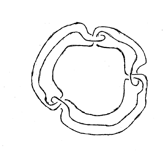
Also, link theory deals with multiple knots together.

The above shows the Borromean Rings, which are three linked knots, no two of which are linked to each other. This is a famous 3-component link.

This blog will mostly focus on the following:
1. non-smooth (and non-piecewise linear) embeddings of the circle into .

These two diagrams are of non-smooth (and non-p. l.) knots; we call these wild knots. Notice how the stitches and arcs get smaller and converge to a point? That point is called a wild point. I will give a precise definition later; for right now we’ll tell you that it is impossible to assign a tangent vector to those points in some well defined way.

2. An arc is the image of into 3 space. The mathematics of smooth (or p. l.) arcs in 3-space is pretty boring. Every smooth or p. l. arc “can be straightened in space” into a straight, boring arc.
On the other hand, the mathematics of wild arcs (think: non-smooth/p. l. ) is every interesting.

The above arc has two wild points (the end points) and can NOT be straightened out in space into a straight arc. We’ll make this concept clear a bit later in another post).

3. Straight lines (a copy of the real line) into open 3-manifolds; we will insist that the “two infinities” of the line go to the “infinities” in the manifold.

In the above, the reader is invited to think of the “line” being embedded in the space where is the standard 2-disk. Think of an infinitely long solid tube or cylinder (like a long pipe).
I will call this Proper Knot Theory; the term “proper” is a technical term, which I will explain here: a continuous map is said to be proper if for all compact sets is compact. Here is an example of a non-proper embedding: consider given by . The inverse image of is not compact.

Equivalence Classes for Knots
In most of knot theory, what is studied is NOT the knots themselves but their “equivalence classes”. For example: the first example of the knot we have had a very specific function to define it. However, if we were to say, take a strand of the knot and move it a little, we’d get a different embedding, but mathematically we’d want to think of it as being “the same as” the original embedding. This makes the subject much more doable. Besides, knot theory is studied mostly because it impacts the study of the topology of 3-manifolds: such spaces are modified by doing operations (called “surgery”) which are often defined as being done along some embedded circle: a knot. In many cases, the objected obtained doesn’t differ “topologically” if the surgery knot is changed by some “motion of space”.

The same principle often applies if a scientist is, say, studying a knotted molecule or DNA strand.

So we need to state the equivalence classes.

Classical Knot Theory (the kind most often done)
Note: sometimes oriented knots are studied (the diagrams have arrows) and sometimes the unoriented knots are studied (no arrows). Sometimes this makes a difference as we shall see later.

The above is an example of an oriented knot diagram.

The most common equivalence class used:
Given two knots (or links) in three space, say, ; we say that is equivalent to $K_2$ if there is a map called an “ambient isotopy” that connects the two. More particularly there exists where:
1. is a homemomorphism of for all .
2. and for some , homeomorphic to the circle.
The above is just a fancy way of saying that we can “deform space” to turn into ; almost never do we worry about finding, say, a formula for .

It turns out that this definition is equivalent to the following simpler definition: are equivalent knots if there is some orientation preserving homeomorphism such that . Needless to say, this is easier to state, but one loses the sense of taking a knotted piece of string and playing with it (which is what you are doing in the first definition).

There is also another type of equivalence that is used: two knots can be declared to be equivalent if there is a homeomorphism (possibly non-orientation preserving) such that .

If is orientation reversing and then and are called mirror images.

So, classical knot theory (the kind most often studied) boils down to four different kinds:
1. oriented knots; mirror images considered equivalent.
2. oriented knots; mirror images NOT automatically considered equivalent.
3. non-oriented knots, mirror images considered equivalent.
4. non-oriented knots, mirror images not automatically considered equivalent.

A knot that is different from a knot with the same image but with a different orientation (arrow direction) is said to be non-invertible.
A knot that is different from its mirror image is said to be chiral.

The trefoil knot: is chiral but invertible (you can reverse the arrows by an orientation preserving homeomorphism)
The figure 8 knot: is NOT chiral and is invertible.

Non-invertible knots exist; here is an example: ()

The astute reader might wonder: “hey, you didn’t say anything about your isotopy or homeomorphism being smooth, piecewise linear or merely topological”. It turns out that in classical knot theory, this is a settled foundational question and therefore unimportant (here and here).

However this issue does appear in other kinds of knot theory, including those we will be discussing.

Wild knots
A knot (link or arc) is said to be tame if it is equivalent to a smooth (or p. l.) knot (equivalence class of choice). If it isn’t, it is called wild.
Note: it isn’t always immediately obvious if an arc is wild or tame; for example, the arc in the upper left hand corner is wild (wild point is the left end point) whereas the the lower right arc (which has separate trefoil knots converging to an endpoint) is actually tame!

We will discuss this later; note that the “infinite trefoil” arc is just on the edge of being wild; were we to add on, say, a straight segment at the left hand endpoint and extend it any finite distance at all, the arc would become wild. That appears to make no sense at all (at first glance) but in a later post I will provide a proof.

We will study wild knots of various kinds; note: it is possible for a knot to be wild at ALL of its points. We’ll get to this in a later post; if you can’t wait, here is an example: consider the following picture, which is supposed to represent a nested series of solid tori, (think: a bagel or doughnut) which are nested inside one another. If we intersect all of these knotted up tori, we end up with a very ill behaved wild knot in 3-space; this knot is wild at all of its points:

I am running out of steam; so in our next installment I’ll talk about different types of equivalence classes for knots in 3 space and for lines (proper knots) in open 3-manifolds. (note: I’ll post this on my research blog, not here).

Slate Post on Math Teaching

Ben Orlin in Slate:

As a math teacher, it’s easy to get frustrated with struggling students. They miss class. They procrastinate. When you take away their calculators, they moan like children who’ve lost their teddy bears. (Admittedly, a trauma.)
Even worse is what they don’t do. Ask questions. Take notes. Correct failing quizzes, even when promised that corrections will raise their scores. Don’t they care that they’re failing? Are they trying not to pass?
There are plenty of ways to diagnose such behavior. Chalk it up to sloth, disinterest, out-of-school distractions—surely those all play a role. But if you ask me, there’s a more powerful and underlying cause.

Math makes people feel stupid. It hurts to feel stupid.

Aw. So he goes on to relate his experience as an undergraduate at Yale, in a topology class:

So I did what most students do. I leaned on a friend who understood things better than I did. I bullied my poor girlfriend (also in the class) into explaining the homework problems to me. I never replicated her work outright, but I didn’t really learn it myself, either. I merely absorbed her explanations enough to write them up in my own words, a misty sort of comprehension that soon evaporated in the sun. (It was the Yale equivalent of my high school students’ worst vice, copying homework. If you’re reading this, guys: Don’t do it!)
I blamed others for my ordeal. Why had my girlfriend tricked me into taking this nightmare class? (She hadn’t.) Why did the professor just lurk in the back of the classroom, cackling at our incompetence, instead of teaching us? (He wasn’t cackling. Lurking, maybe, but not cackling.) Why did it need to be stupid topology, instead of something fun? (Topology is beautiful, the mathematics of lava lamps and pottery wheels.) And, when other excuses failed, that final line of defense: I hate this class! I hate topology!

You can read the rest.
Here is his conclusion:

Teachers have such power. He could have crushed me if he wanted.
He didn’t, of course. Once he recognized my infantile state, he spoon-fed me just enough ideas so that I could survive the lecture. I begged him not to ask me any tough questions during the presentation—in effect, asking him not to do his job—and with a sigh he agreed.
I made it through the lecture, graduated the next month, and buried the memory as quickly as I could.
Looking back, it’s amazing what a perfect specimen I was. I manifested every symptom that I now see in my own students:
Muddled half-comprehension.
Fear of asking questions.
Shyness about getting the teacher’s help.
Badgering a friend instead.
Copying homework.
Excuses; blaming others.
Procrastination.
Anxiety about public failure.
Terror of the teacher’s judgment.
Feeling incurably stupid.
Not wanting to admit any of it.
It’s surprisingly hard to write about this, even now. Mathematical failure—much like romantic failure—leaves us raw and vulnerable. It demands excuses.
I tell my story to illustrate that failure isn’t about a lack of “natural intelligence,” whatever that is. Instead, failure is born from a messy combination of bad circumstances: high anxiety, low motivation, gaps in background knowledge. Most of all, we fail because, when the moment comes to confront our shortcomings and open ourselves up to teachers and peers, we panic and deploy our defenses instead. For the same reason that I pushed away topology, struggling students push me away now.
Not understanding topology doesn’t make me stupid. It makes me bad at topology.

Ok.

First of all: it IS in part, about natural intelligence. The really smart math people, in general, don’t have trouble with undergraduate math classes, even those at Yale. I mean, of course, REALLY smart people (no, I am not one of those. 🙂 ).

Now he has an interesting observation about student “employing defenses”; at least some of them do.

But there are a host of other reasons too: some just don’t like the material, some ARE lazy (e. g., they won’t do what isn’t fun) and yes, some aren’t up to the task intellectually. Seriously: there are some subjects that many will never be able to master, even at an undergraduate level.

But one issue: someone on Facebook made the following comment:

Oh boohoo. If you’re bad at something you either make an attempt to improve at it or direct your attention to things you’re better at. Everyone is not good at everything and feeling stupid is not something people should be protected from. If you don’t get told you make mistakes or aren’t made to realize that some things take effort then you’re not improving. Learning disabilities aside, especially in higher math, the kids that are failing aren’t showing up to anything, aren’t doing the work, aren’t asking questions, aren’t studying and they don’t repeat to try and do better the next time. Children need to know what failure feels like (and math teachers were children and they do all likely know what failure feels like) so that they learn to try.

Emphasis mine.

My Opinion:
1. There are things that are too difficult for most of us to learn (e. g. quantum field theory).
2. It is useful to have a grasp of one’s intellectual limitations. All too often I see average people dismissing expert findings because those findings “don’t make sense to them.” People need MORE intellectual humility, not less of it.
3. If you haven’t failed at something, then you haven’t tried enough difficult things.

That said: this article is useful because it does give at least one angle of approach that might work with some students.

Unsolicited advise to young professors at heavy teaching load universities: Go to Research Conferences anyway!

This is coming to you from Ames, Iowa at the Spring American Mathematical Society Meeting. I am here to attend the sessions on the Topology of 3-dimensional manifolds.

Note: I try to go to conferences regularly; I have averaged about 1 conference a year. Sometimes, the conference is a MAA Mathfest conference. These ARE fun and refreshing. But sometimes (this year), I go to a research oriented conference.

I’ll speak for myself only.

Sometimes, these can be intimidating. Though many of the attendees are nice, cordial and polite, the fact is that many (ok, almost all of them) are either the best graduate students or among the finest researchers in the world. The big names who have proved the big theorems are here. They earn their living by doing cutting edge research and by guiding graduate students through their research; they are not spending hours and hours convincing students that .

So, the talks can be tough. Sure, they do a good job, but remember that most of the audience is immersed in this stuff; they don’t have to review things like “normal surface theory” or “Haken manifold”.

Therefore, it is VERY easy to start lamenting (internally) “oh no, I am by far the dumbest one here”. That, in my case, IS true, but it is unimportant.
What I found is that, if I pay attention to what I can absorb, I can pick up a technique here and there, which I can then later use in my own research. In fact, just today, I picked up something that might help me with a problem that I am pondering.

Also, the atmosphere can be invigorating!

I happen to enjoy the conferences that are held on university campuses. There is nothing that gets my intellectual mood pumped up more than to hang around the campus of a division I research university. For me, there is nothing like it.

This conference
A few general remarks:
1. I didn’t realize how pretty Iowa State University is. I’d rank it along with the University of Tennessee as among the prettiest campuses that I’ve ever seen.

2. As far as the talks: one “big picture” technique that I’ve seen used again and again is the technique of: take an abstract set of objects (say, the Seifert Surfaces of a knot; say of minimal genus. Then to each, say, ambient isotopy class of Seifert Surface, assign a vertex of a graph or simplicial complex. Then group the vertices together either by a segment (in some settings) or a simplex (if, in one setting, the Seifert Surfaces admit disjoint representatives). Then one studies the complex or the graph.

In one of the talks (talking about essential closed surfaces in the complement of a knot), one assigned such things to the vertex of a graph (dendron actually) and set up an algorithm to search along such a graph; it turns out that is one starts near the top of this dendron, one gains the opportunity to prune lower branches of the group by doing the calculation near the top.

Sidenote
The weather couldn’t be better; I found time over lunch to do a 5.7 mile run near my hotel. The run was almost all on bike paths (albeit a “harder” surface than I’d like).

Personal Note

After a LONG drought I finally got another paper accepted for publication.

I teach at a 11-12 teaching load institution and therefore don’t publish at nearly the rate that a professor at a research institution does.

I’ll admit that I went through a crisis of confidence after a rejection or two; I am going to celebrate this one. 🙂

And yes, I have another paper almost ready to go.

Google Doodle 15 April 2013

Which famous mathematician is being honored? 🙂

Calculus and Analysis: the power of examples

In my non-math life I am an avid runner and walker. Ok, my enthusiasm for these sports greatly excedes my talent and accomplishments for these sports; I once (ONCE) broke 40 minutes for the 10K run and that was in 1982; the winner (a fellow named Bill Rodgers) won that race and finished 11 minutes ahead of me that day! 🙂 Now I’ve gotten even slower; my fastest 10K is around 53 minutes and I haven’t broken 50 since 2005. 😦

But alas I got a minor bug and had to skip today’s planned races; hence I am using this morning to blog about some math.

Real Analysis and Calculus
I’ve said this before and I’ll say it again: one of my biggest struggles with real analysis and calculus was that I often didn’t see the point of the nuances in the proof of the big theorems. My immature intuition was one in which differentiable functions were, well, analytic (though I didn’t know that was my underlying assumption at the time). Their graphs were nice smooth lines, though I knew about corners (say, at .

So, it appears to me that one of the way we can introduce the big theorems (along with the nuances) is to have a list of counter examples at the ready and be ready to present these PRIOR to the proof; that way we can say “ok, HERE is why we need to include this hypothesis” or “here is why this simple minded construction won’t work.”

So, what are my favorite examples? Well, one is the function is a winner. This gives an example of a function that is not analytic (on any open interval containing 0 ).

The family of examples I’d like to focus on today is , fixed, .

Note: henceforth, when I write I’ll let it be understood that I mean the conditional function that I wrote above.

Use of this example:
1. Squeeze theorem in calculus: of course, ; this is one time we can calculate a limit without using a function which one can merely “plug in”. It is easy to see that .

2. Use of the limit definition of derivative: one can see that ; this is one case where we can’t merely “calculate”.

3. provides an example of a function that is differentiable at the origin but is not continuously differentiable there. It isn’t hard to see why; away from 0 the derivative is and the limit as approaches zero exists for the first term but not the second. Of course, by upping the power of one can find a function that is times differentiable at the origin but not continuously differentiable.

4. The proof of the chain rule. Suppose is differentiable at and is differentiable at . Then we know that is differentiable at and the derivative is . The “natural” proof (say, for non-constant near looks at the difference quotient: which works fine, so long as . So what could possibly go wrong; surely the set of values of for which for a differentiable function is finite right? 🙂 That is where comes into play; this equals zero at an infinite number of points in any neighborhood of the origin.

Hence the proof of the chain rule needs a workaround of some sort. This is a decent article on this topic; it discusses the usual workaround: define . Then it is easy to see that since the second factor of the last term is zero when and the limit of exists at .

Of course, one doesn’t have to worry about any of this if one introduces the “grown up” definition of derivative from the get-go (as in: best linear approximation) and if one has a very gifted class, why not?

5. The concept of “bounded variation” and the Riemann-Stiltjes integral: given functions over some closed interval and partitions look at upper and lower sums of and if the upper and lower sums converge as the width of the partions go to zero, you have the integral . But this works only if has what is known as “bounded variation”: that is, there exists some number such that for ALL partitions . Now if is differentiable with a bounded derivative on (e. g. is continuously differentiable on then it isn’t hard to see that had bounded variation. Just let be a bound for and then use the Mean Value Theorem to replace each by and the result follows easily.

So, what sort of function is continuous but NOT of bounded variation? Yep, you guessed it! Now to make the bookkeeping easier we’ll use its sibling function: . 🙂 Now consider a partition of the following variety: . Example: say . Compute the variation: . This leads to trouble as this sum has no limit as we progress with more points in the sequence of partitions; we end up with a divergent series (the Harmonic Series) as one term as points are added to the partition.

6. The concept of Absolute Continuity: this is important when one develops the Fundamental Theorem of Calculus for the Lebesgue integral. You know what it means for to be continuous on an interval. You know what it means for to be uniformly continuous on an interval (basically, for the whole interval, the same works for a given no matter where you are, and if the interval is a closed one, an easy “compactness” argument shows that continuity and uniform continuity are equivalent. Absolute continuity is like uniform continuity on steroids. I’ll state it for a closed interval: is absolutely continuous on an interval if, given any there is a such that for where are pairwise disjoint intervals. An example of a function that is continuous on a closed interval but not absolutely continuous? Yes; on any interval containing is an example; the work that we did in paragraph 5 works nicely; just make the intervals pairwise disjoint.

Fun for my Facebook Friends

Fun question one: can anyone see the relation between the following three figures? Note: I made a (sort of subtle) mistake in one of them….the one where the graph lines are showing)

Fun question two (a bit harder):

What is the relation between these figures?

And for the win: what is going on here? (this is ambiguous)

Ok, I’ll help you with the last one: imagine this process (one solid torus (think: doughnut or bagel) inside a larger one, and repeat this process (think: those Russian dolls that are nested). If you then take the infinite intersection, you get a simple closed curve (not obvious) that is so badly embedded, it fails to pierce a disk at any of its points (and certainly fails to have a tangent vector anywhere).