I’ve used the presentation in the our Probability and Statistics text; it is appropriate given that many of our students haven’t seen the Fourier Transform. But this presentation is excellent.
Upshot: use the convolution to derive the density function for (independent, identically distributed random variables of finite variance), assume mean is zero, variance is 1 and divide by to obtain the variance of the sum to be 1. Then use the Fourier transform on the whole thing (the normalized version) to turn convolution into products, use the definition of Fourier transform and use the Taylor series for the terms, discard the high order terms, take the limit as goes to infinity and obtain a Gaussian, which, of course, inverse Fourier transforms to another Gaussian.
For us, calculus III is the most rushed of the courses, especially if we start with polar coordinates. Getting to the “three integral theorems” is a real chore. (ok, Green’s, Divergence and Stoke’s theorem is really just but that is the subject of another post)
But watching this lecture made me wonder: should I say a few words about how to calculate a convolution integral?
In the context of Fourier Transforms, the convolution integral is defined as it was in analysis class: . Typically, we insist that the functions be, say, and note that it is a bit of a chore to show that the convolution of two functions is ; one proves this via the Fubini-Tonelli Theorem.
(The straight out product of two functions need not be ; e.g, consider for and zero elsewhere)
So, assuming that the integral exists, how do we calculate it? Easy, you say? Well, it can be, after practice.
But to test out your skills, let be the function that is for and zero elsewhere. So, what is ???
So, it is easy to see that only assumes the value of on a specific region of the plane and is zero elsewhere; this is just like doing an iterated integral of a two variable function; at least the first step. This is why it fits well into calculus III.
for the following region:
This region is the parallelogram with vertices at .
Now we see that we can’t do the integral in one step. So, the function we are integrating has the following description:
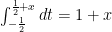
So the convolution integral is for and for .
That is, of course, the tent map that we described here. The graph is shown here:
So, it would appear to me that a good time to do a convolution exercise is right when we study iterated integrals; just tell the students that this is a case where one “stops before doing the outside integral”.
The context: one is showing that the Fourier transform of the convolution of two functions is the product of the Fourier transforms (very similar to what happens in the Laplace transform); that is where
So, during this lecture, Osgood shows that ; that is, this modified Gaussian function is “its own Fourier transform”.
I’ll sketch out what he did in the lecture at the end of this post. But just for fun (and to make a point) I’ll give a method that uses an elementary residue integral.
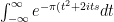
Both methods start by using the definition:
Method 1: combine the exponential functions in the integrand:
. Now complete the square to get:
Now factor out the factor involving alone and write as a square:
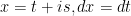
Now, make the substitution to obtain:
Now we show that the above integral is really equal to
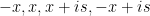
To show this, we perform along the retangular path : and let
Now the integral around the contour is 0 because is analytic.
We wish to calculate the negative of the integral along the top boundary of the contour. Integrating along the bottom gives 1.
As far as the sides: if we fix we note that and the magnitude goes to zero as So the integral along the vertical paths approaches zero, therefore the integrals along the top and bottom contours agree in the limit and the result follows.
Method 2: The method in the video
This uses “differentiation under the integral sign”, which we talk about here.
Stat with and note
Now we do integration by parts: and the integral becomes:
Now the first term is zero for all values of as . The second term is merely:
.
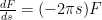
So we have shown that which is a differential equation in which has solution (a simple separation of variables calculation will verify this). Now to solve for the constant note that .
The result follows.
Now: which method was easier? The second required differential equations and differentiating under the integral sign; the first required an easy residue integral.
By the way: the video comes from an engineering class. Engineers need to know this stuff!
I’ve been following these excellent lectures by Professor Brad Osgood of Stanford. As an aside: yes, he is dynamite in the classroom, but there is probably a reason that Stanford is featuring him. 🙂
And yes, his style is good for obtaining a feeling of comradery that is absent in my classroom; at least in the lower division “service” classes.
This lecture takes us from Fourier Series to Fourier Transforms. Of course, he admits that the transition here is really a heuristic trick with symbolism; it isn’t a bad way to initiate an intuitive feel for the subject though.
However, the point of this post is to offer a “algebra of calculus trick” for dealing with the sort of calculations that one might encounter.
By the way, if you say “hey, just use a calculator” you will be BANNED from this blog!!!! (just kidding…sort of. 🙂 )
So here is the deal: let represent the tent map: the support of is and it has the following graph:
The formula is:
So, the Fourier Transform is
Now, this is an easy integral to do, conceptually, but there is the issue of carrying constants around and being tempted to make “on the fly” simplifications along the way, thereby leading to irritating algebraic errors.
So my tip: just let and do the integrals:
and substitute and simplify later:
Now the integrals become:
These are easy to do; the first is merely and the next two have the same anti-derivative which can be obtained by a “integration by parts” calculation: ; evaluating the limits yields:
Add the first integral and simplify and we get: . NOW use and we have the integral is by Euler’s formula.
Now we need some trig to get this into a form that is “engineering/scientist” friendly; here we turn to the formula: so so our answer is which is often denoted as as the “normalized” function is given by (as we want the function to have zeros at integers and to “equal” one at (remember that famous limit!)
So, the point is that using made the algebra a whole lot easier.
Now, if you are shaking your head and muttering about how this calculation was crude that that one usually uses “convolution” instead: this post is probably too elementary for you. 🙂


 but that is the subject of another post)
 . Typically, we insist that the functions be, say,
  and note that it is a bit of a chore to show that the convolution of two
  for
for ![x \in (0,1]](https://s0.wp.com/latex.php?latex=x+%5Cin+%280%2C1%5D+&bg=ffffff&fg=000000&s=0&c=20201002) and zero elsewhere)
and zero elsewhere)  be the function that is
  for
for ![x \in [\frac{-1}{2}, \frac{1}{2}]](https://s0.wp.com/latex.php?latex=x+%5Cin+%5B%5Cfrac%7B-1%7D%7B2%7D%2C+%5Cfrac%7B1%7D%7B2%7D%5D+&bg=ffffff&fg=000000&s=0&c=20201002) and zero elsewhere. So, what is
and zero elsewhere. So, what is  ???
??? only assumes the value of
  plane and is zero elsewhere; this is just like doing an iterated integral of a two variable function; at least the first step. This is why it fits well into calculus III.
 for the following region:
 .
. 
 has the following description:
![f(x-t)f(t)=\left\{\begin{array}{c} 1,x \in [-1,0], -\frac{1}{2} t \le \frac{1}{2}+x \\ 1 ,x\in [0,1], -\frac{1}{2}+x \le t \le \frac{1}{2} \\ 0 \text{ elsewhere} \end{array}\right.](https://s0.wp.com/latex.php?latex=f%28x-t%29f%28t%29%3D%5Cleft%5C%7B%5Cbegin%7Barray%7D%7Bc%7D+1%2Cx+%5Cin+%5B-1%2C0%5D%2C+-%5Cfrac%7B1%7D%7B2%7D+t+%5Cle+%5Cfrac%7B1%7D%7B2%7D%2Bx+%5C%5C+1+%2Cx%5Cin+%5B0%2C1%5D%2C+-%5Cfrac%7B1%7D%7B2%7D%2Bx+%5Cle+t+%5Cle+%5Cfrac%7B1%7D%7B2%7D+%5C%5C+0+%5Ctext%7B+elsewhere%7D+%5Cend%7Barray%7D%5Cright.++&bg=ffffff&fg=000000&s=0&c=20201002)
 for
for  and
and  for
for ![x \in [0,1]](https://s0.wp.com/latex.php?latex=x+%5Cin+%5B0%2C1%5D+&bg=ffffff&fg=000000&s=0&c=20201002) .
.
 where
where 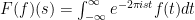 provided the integral converges.
  ; one can check that
  . One way is to use the fact that
  and do the substitution
  ; of course one should be able to
  ; that is, this modified Gaussian function is “its own Fourier transform”.
 . Now complete the square to get:
 alone and write as a square:
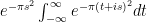
 to obtain:

 along the retangular path
  :
:  and let

 is analytic.
  and the magnitude goes to zero as
 and the integral becomes:
 . The second term is merely:
 .
. which is a differential equation in
  (a simple separation of variables calculation will verify this). Now to solve for the constant
  note that
 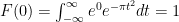 .
.  represent the tent map: the support of
  is
is ![[-1,1]](https://s0.wp.com/latex.php?latex=%5B-1%2C1%5D+&bg=ffffff&fg=000000&s=0&c=20201002) and it has the following graph:
and it has the following graph:![f(x)=\left\{\begin{array}{c} x+1,x \in [-1,0) \\ 1-x ,x\in [0,1] \\ 0 \text{ elsewhere} \end{array}\right.](https://s0.wp.com/latex.php?latex=f%28x%29%3D%5Cleft%5C%7B%5Cbegin%7Barray%7D%7Bc%7D+x%2B1%2Cx+%5Cin+%5B-1%2C0%29+%5C%5C+1-x+%2Cx%5Cin+%5B0%2C1%5D+%5C%5C+0+%5Ctext%7B+elsewhere%7D+%5Cend%7Barray%7D%5Cright.++&bg=ffffff&fg=000000&s=0&c=20201002)

 and do the integrals:
 and substitute and simplify later:
 and the next two have the same anti-derivative which can be obtained by a “integration by parts” calculation:
  ; evaluating the limits yields:
 . NOW use
  and we have the integral is
  by Euler’s formula.
 so
so  so our answer is
  which is often denoted as
  as
as  function
 (as we want the function to have zeros at integers and to “equal” one at
  (remember that famous limit!)
 made the algebra a whole lot easier.