existence and uniqueness | College Math Teaching

October 1, 2014

Osgood’s uniqueness theorem for differential equations

Filed under: advanced mathematics, analysis, calculus, differential equations — Tags: existence and uniqueness, Osgood's uniqueness theorem — collegemathteaching @ 1:59 am

I am teaching a numerical analysis class this semester and we just started the section on differential equations. I want them to understand when we can expect to have a solution and when a solution satisfying a given initial condition is going to be unique.

We had gone over the “existence” theorem, which basically says: given $y' = f(x,y)$ and initial condition $y(x_0) = y_0$ where $(x_0,y_0) \in int(R)$ where $R$ is some rectangle in the $x,y$ plane, if $f(x,y)$ is a continuous function over $R$ , then we are guaranteed to have at least one solution to the differential equation which is guaranteed to be valid so long as $(x, y(x)$ stays in $R$ .

I might post a proof of this theorem later; however an outline of how a proof goes will be useful here. With no loss of generality, assume that $x_0 = 0$ and the rectangle has the lines $x = -a, x = a$ as vertical boundaries. Let $\phi_0 = f(0, y_0)x$ , the line of slope $f(0, y_0)$ . Now partition the interval $[-a, a]$ into $-a, -\frac{a}{2}, 0, \frac{a}{2}, a$ and create a polygonal path as follows: use slope $f(0, y_0)$ at $(0, y_0)$ , slope $f(\frac{a}{2}, y_0 + \frac{a}{2}f(0, y_0))$ at $(\frac{a}{2}, y_0 + \frac{a}{2}f(0, y_0))$ and so on to the right; reverse this process going left. The idea: we are using Euler’s differential equation approximation method to obtain an initial piecewise approximation. Then do this again for step size $\frac{a}{4},$

In this way, we obtain an infinite family of continuous approximation curves. Because $f(x,y)$ is continuous over $R$ , it is also bounded, hence the curves have slopes whose magnitude are bounded by some $M$ . Hence this family is equicontinuous (for any given $\epsilon$ one can use $\delta = \frac{\epsilon}{M}$ in continuity arguments, no matter which curve in the family we are talking about. Of course, these curves are uniformly bounded, hence by the Arzela-Ascoli Theorem (not difficult) we can extract a subsequence of these curves which converges to a limit function.

Seeing that this limit function satisfies the differential equation isn’t that hard; if one chooses $t, s \in (-a.a)$ close enough, one shows that $| \frac{\phi_k(t) - \phi_k(s)}{(t-s)} - f(t, \phi(t))| 0$ where $|f(x,y_1)-f(x,y_2)| \le K|y_1-y_2|$ then the differential equation $y'=f(x,y)$ has exactly one solution where $\phi(0) = y_0$ which is valid so long as the graph $(x, \phi(x) )$ remains in $R$ .

Here is the proof: $K > 0$ where $|f(x,y_1)-f(x,y_2)| \le K|y_1-y_2| < 2K|y_1-y_2|$ . This is clear but perhaps a strange step.
But now suppose that there are two solutions, say $y_1(x)$ and $y_2(x)$ where $y_1(0) = y_2(0)$ . So set $z(x) = y_1(x) -y_2(x)$ and note the following: $z'(x) = y_1(x) - y_2(x) = f(x,y_1)-f(x,y_2)$ and $|z'(x)| = |f(x,y_1)-f(x,y_2)| 0$ . A Mean Value Theorem argument applied to $z$ means that we can assume that we can select our $x_1$ so that $z' > 0$ on that interval (since $z(0) = 0$ ).

So, on this selected interval about $x_1$ we have $z'(x) < 2Kz$ (we can remove the absolute value signs.).

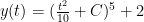
Now we set up the differential equation: $Y' = 2KY, Y(x_1) = z(x_1)$ which has a unique solution $Y=z(x_1)e^{2K(x-x_1)}$ whose graph is always positive; $Y(0) = z(x_1)e^{-2Kx_1}$ . Note that the graphs of $z(x), Y(x)$ meet at $(x_1, z(x_1))$ . But $z'(x) 0$ where $z(x_1 - \delta) > Y(x_1 - \delta)$ .

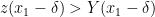But since $z(0) = 0 z'(x)$ on that interval.

So, no such point $x_1$ can exist.

Note that we used the fact that the solution to 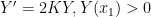$Y' = 2KY, Y(x_1) > 0$ is always positive. Though this is an easy differential equation to solve, note the key fact that if we tried to separate the variables, we’d calculate $\int_0^y \frac{1}{Kt} dt$ and find that this is an improper integral which diverges to positive $\infty$ hence its primitive cannot change sign nor reach zero. So, if we had $Y' =2g(Y)$ where $\int_0^y \frac{1}{g(t)} dt$ is an infinite improper integral and $g(t) > 0$ , we would get exactly the same result for exactly the same reason.

Hence we can recover Osgood’s Uniqueness Theorem which states:

If $f(x,y)$ is continuous on $R$ and for all $(x, y_1), (x, y_2) \in R$ we have a $K > 0$ where $|f(x,y_1)-f(x,y_2)| \le g(|y_1-y_2|)$ where $g$ is a positive function and $\int_0^y \frac{1}{g(t)} dt$ diverges to $\infty$ at $y=0$ then the differential equation $y'=f(x,y)$ has exactly one solution where $\phi(0) = y_0$ which is valid so long as the graph $(x, \phi(x) )$ remains in $R$ .

Comments (6)

September 23, 2014

Ok, what do you see here? (why we don’t blindly trust software)

Filed under: analysis, applied mathematics, calculus, differential equations — Tags: caveats, existence and uniqueness, mathematical software — collegemathteaching @ 7:09 pm

I had Dfield8 from MATLAB propose solutions to $y' = t(y-2)^{\frac{4}{5}}$ meeting the following initial conditions:

$y(0) = 0, y(0) = 3, y(0) = 2$ .

Now, of course, one of these solutions is non-unique. But, of all of the solutions drawn: do you trust ANY of them? Why or why not?

Note: you really don’t have to do much calculus to see what is wrong with at least one of these. But, if you must know, the general solution is given by $y(t) = (\frac{t^2}{10} +C)^5 + 2$ (and, of course, the equilibrium solution $y = 2$ ). But that really doesn’t provide more information that the differential equation does.

By the way, here are some “correct” plots of the solutions, (up to uniqueness)

College Math Teaching

October 1, 2014

Osgood’s uniqueness theorem for differential equations

September 23, 2014

Ok, what do you see here? (why we don’t blindly trust software)

Categories

Blogroll

Archives

Top Clicks

Top Posts