I am thinking about doing a series of videos on the annoying but necessary calculations one encounters in basic calculus based statistics classes. I made the first video, which I am posting here. Below I post the whiteboards (too lazy to typeset).
The problem (from Larson’s Calculus, an Applied Approach, 10’th edition, Section 7.8, no. 18 in my paperback edition, no. 17 in the e-book edition) does not seem that unusual at a very quick glance:
if you have a hard time reading the image. AND, *if* you just blindly do the formal calculations:
which is what the text has as “the answer.”
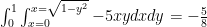
But come on. We took a function that was negative in the first quadrant, integrated it entirely in the first quadrant (in standard order) and ended up with a positive number??? I don’t think so!
Indeed, if we perform which is far more believable.
So, we KNOW something is wrong. Now let’s attempt to sketch the region first:
Oops! Note: if we just used the quarter circle boundary we obtain
The 3-dimensional situation: we are limited by the graph of the function, the cylinder and the planes ; the plane is outside of this cylinder. (from here: the red is the graph of
Now think about what the “formal calculation” really calculated and wonder if it was just a coincidence that we got the absolute value of the integral taken over the rectangle
It is not a surprise that my posts here have fallen off by quite a bit. Part of it is that I’ve been assigned a lot of teaching of courses that I have to do extra preparation for.
And yes, the nature of the job has changed. Student body is more or less the same size, but we’ve been reduced from 15 tenure track lines to 9. This means: larger size sections, more students to advise (per professor) and less selection among upper division classes.
Ok, jobs change and I am not treated that poorly. Yes, I wish our classrooms had better IT structure and we didn’t have so many per section.
But the real issue is the loss of tenure track lines and the reliance on visitors.
The number of applicants, at least for the temporary jobs, has dropped by an order of 10.
What is going on, I think: university administrations have embraced, IN PART, a “run it like a business” attitude.
So, they see small class sizes as wasted resources. They see work week “down time” to think about scholarship OR to think about how to approach/teach a class as wasted time. I can’t remember the time I last thought about mathematics during an academic year.
And frankly, I am often not tempted: IF one gets a bit of time to do math, subsequent open slots are often filled by duties, student needs (more students = more exceptional cases; e. g. accidents, illnesses, etc.) and by the time I can get back to it, I’ve often forgotten my train of thought.
And so, what is offered to those who apply for our jobs? Mostly, it is packed schedules, packed classrooms and not much job security (yes, tenure track faculty can be let go for reasons other than performance).
And back to the “run it like a business model”: we want business demands on potential workers, but we don’t want to compete with respect to compensation.
In my day: I took less money than I could have made outside, in return for being able to do a bit of scholarship and have a bit of fun with classes and enjoy a “family like” atmosphere with extra job security.
That has been taken away; only the “lower pay” remains, and new job seekers are savvy enough to see that.
If we want to “run it like a business”, we need to compete with businesses for young talent, and we aren’t doing that.
My guess: things will be very grim over the next half-decade to a decade, at least at the non-R1 universities.
Of course, for readers of this blog: easy-peasy. so the integral is transformed into and so we’ve entered the realm of rational functions. Ok, ok, there is some work to do.
But for now, notice what is really doing on: we have a function under the radical that has an inverse function (IF we are careful about domains) and said inverse function has a derivative which is a rational function
More shortly: let be such that then:
gets transformed: and then and the integral becomes which is a rational function integral.
I made a short video; no, I did NOT have “risk factor”/”age group” breakdown, but the overall point is that vaccines, while outstanding, are NOT a suit of perfect armor.
Upshot: I used this local data:
The vaccination rate of the area is slightly under 50 percent; about 80 percent for the 65 and up group. But this data doesn’t break it down among age groups so..again, this is “back of the envelope”:
or about 77 percent efficacy with respect to hospitalization, and or 93.75 percent with respect to ending up in the ICU.
Again, the efficacy is probably better than that because of the lack of risk factor correction.
Note: the p-value for the statistical test of vaccines have no effect on hospitalization” vs. “effect” is
Background: we are a “primarily undergraduate” non-R1 institution. We do not offer math master’s degrees but the engineering college does.
Me: old full professor who has either served on or chaired several search committees.
I’ll break this post down into the two types of jobs we are likely to offer: Tenure Track lecturer
Tenure Track Assistant Professor.
Lecturer
No research requirement; this job consists of teaching 12 hour loads of lower division mathematics classes, mostly “business calculus and below”; college algebra and precalculus will be your staples. There will be some service work too.
What we are looking for:
Evidence that you have taught lower division courses (college algebra, precalculus, maybe “baby stats”) successfully. Yes, it is great that you were the only postdoc asked to teach a course on differentiable manifolds or commutative ring theory but that is not relevant to this job.
So hopefully you have had taught these courses in the past (several times) and your teaching references talk about how well you did in said courses; e. g. students did well in said courses, went on to the next course prepared, course was as well received as such a course can be, etc. If you won a teaching award of some kind (or nominated for one), that is good to note. And, in this day and age..how did the online stuff go?
Teaching statement: ok, I am speaking for myself, but what I look for is: did you evaluate your own teaching? What did you try? What problems did you notice? Where could you have done better, or what could you try next time? Did you discuss your teaching with someone else? All of those things stand out to me. And yes, that means recognizing that what you tried didn’t work this time…and that you have a plan to revise it..or DID revise it. This applies to the online stuff too.
Diversity Statement Yes, that is a relatively new requirement for us. What I look for: how do you adjust to having some cultural variation in your classroom? Here are examples of what I am talking about:
We usually get students from the suburbs who are used to a “car culture.” So, I often use the car speedometer as something that gives you the derivative of the car’s position. But I ended up with a student from an urban culture and she explained to me that she and her friends took public transportation everywhere…I had to explain what a speedometer was. It was NOT walking around knowledge.
Or: there was a time when I uploaded *.doc files to our learning management system. It turns out that not all students have Microsoft word; taking a few seconds to make them *.pdf files made it a LOT easier for them.
Other things: not everyone gets every sports analogy, gambling analogy (cards, dice, etc.) so be patient when explaining the background for such examples.
Also: a discussion on how one adjusts for the “gaps” in preparation that students have is a plus; a student can place into a course but have missing topics here and there. And the rigor of the high school courses may well vary from student to student; some might expect to be given a “make up” exam if they do poorly on an exam; another might have been used to be given credit for totally incorrect work (I’ve seen both).
Also: if you’ve tutored or volunteered to help a diverse group of students, be sure to mention that (e. g. maternity homes, sports teams, urban league, or just the tutoring center, etc.)
Transcript: yes, we require it, but what we are looking for is breath for the lecturer’s job: the typical is to have three of the following covered: “algebra, analysis, topology, probability, statistics, applied math”
Cover letter: Something that shows that you know the type of job we are offering is very helpful; if you state that you “want to direct undergraduate research”, well, our lecturer job will be a huge letdown.
Assistant Professor
This job will involve 9-12 hours teaching; 10-11 is typical and we do have a modest research requirement. 2-3 papers in solid journals will be sufficient for tenure; you might not want to have your heart set on an Annals of Math publication. If you do get one, you won’t be with us for long anyway. There is also advising and service work.
What we are looking for: teaching: we want some evidence that you can teach the courses typically taught by our department. This means some experience in calculus/business calculus for our math track, and statistics for our statistics track. For this job, some evidence for upper division is a plus, but not required nor even expected; is is an extra “nice to have.”
But it is all but essential that your teaching references talks about your performance in teaching lower division classes (calculus or below); if all you have is “the functional analysis students loved him/her”, that is not helpful. Being observed while teaching a lower division course is all but essential.
Teaching and Diversity statement : same as for the lecturer job. An extra: did you have any involvement with the math club?
Research: the thing we are looking for is: will you “die on the vine” or not? Having a plan: “I intend to move from my dissertation in this direction” is a plus, as is having others to collaborate with (though collaboration isn’t necessary). Also, a statement from your advisor that you can work INDEPENDENTLY ..that is, you can find realistic problems to work on and do NOT need hand holding, is a major plus. You are likely to be somewhat isolated here. And of course, loving mathematics is essential with us. Not all candidates do..if you see your dissertation as a task you had to do to get the credential then our job isn’t for you.
Another plus: having side projects that an undergraduate can work on is a plus. We do have some undergraduate research but that won’t be the bulk of the job.
This is “part 2” of a previous post about series. Once again, this is not designed for students seeing the material for the first time.
I’ll deal with general power series first, then later discuss Taylor Series (one method of obtaining a power series).
General Power Series Unless otherwise stated, we will be dealing with series such as though, of course, a series can expanded about any point in the real line (e. g. ) Note: unless it is needed, I’ll be suppressing the index in the summation sign.
So, IF we have a function ..
what do we mean by this and what can we say about it?
The first thing to consider, of course, is convergence. One main fact is that the open interval of convergence of a power series centered at 0 is either: 1. Non existent …series converges at only (e. g. ; try the ratio test) or
2. Converges absolutely on for some and diverges for all (like a geometric series) (anything possible for ) or
3. Converges absolutely on the whole real line.
Many texts state this result but do not prove it. I can understand as this result is really an artifact of calculus of a complex variable. But it won’t hurt to sketch out a proof at least for the “converge” case for so I’ll do that.
So, let’s assume that converges (either absolute OR conditional ) So, by the divergence test, we know that the sequence of terms . So we can find some index such that
So write: and converges absolutely for . The divergence follows from a simple “reversal of the inequalities (that is, if the series diverged at ).
Though the relation between real and complex variables might not be apparent, it CAN be useful. Here is an example: suppose one wants to find the open interval of convergence of, say, the series representation for ? Of course, the function itself is continuous on the whole real line. But to find the open interval of convergence, look for the complex root of that is closest to zero. That would be so the interval is
So, what about a function defined as a power series?
For one, a power series expansion of a function at a specific point (say, ) is unique:
Say on the interval of convergence, then substituting yields . So subtract from both sides and get: . Now assuming one can “factor out an x” from both sides (and you can) we get , etc.
Yes, this should have property been phrased as a limit and I’ve yet to show that is continuous on its open interval of absolute convergence.
Now if you say “doesn’t that follow from uniform convergence which follows from the Weierstrass M test” you’d be correct…and you are probably wasting your time reading this.
Now if you remember hearing those words but could use a refresher, here goes:
We want for sufficiently close AND both within the open interval of absolute convergence, say Choose where and such that and where (these are just polynomials).
The rest follows:
Calculus On the open interval of absolute convergence, a power series can be integrated term by term and differentiated term by term. Neither result, IMHO, is “obvious.” In fact, sans extra criteria, for series of functions, in general, it is false. Quickly: if you remember Fourier Series, think about the Fourier series for a rectangular pulse wave; note that the derivative is zero everywhere except for the jump points (where it is undefined), then differentiate the constituent functions and get a colossal mess.
Differentiation: most texts avoid the direct proof (with good reason; it is a mess) but it can follow from analysis results IF one first shows that the absolute (and uniform) convergence of implies the absolute (and uniform) convergence of
So, let’s start here: if is absolutely convergent on then so is .
Here is why: because we are on the open interval of absolute convergence, WLOG, assume and find where is also absolutely convergent. Now, note that so the series converges by direct comparison on which establishes what we wanted to show.
Of course, this doesn’t prove that the expected series IS the derivative; we have a bit more work to do.
Again, working on the open interval of absolute convergence, let’s look at:
Now, we use the fact that is absolutely convergent on and given any we can find so that for between and
So let’s do that: pick and then note:
Now apply the Mean Value Theorem to each term in the second term:
where each is between and . By the choice of the second term is less than , which is arbitrary, and the first term is the first terms of the “expected” derivative series.
So, THAT is “term by term” differentiation…and notice that we’ve used our hypothesis …almost all of it.
Term by term integration
Theoretically, integration combines easier with infinite summation than differentiation does. But given we’ve done differentiation, we can then do anti-differentiation by showing that converges and then differentiating.
But let’s do this independently; it is good for us. And we’ll focus on the definite integral.
(of course, )
Once again, choose so that
Then and this is less than (or equal to)
But is arbitrary and so the result follows, for definite integrals. It is an easy exercise in the Fundamental Theorem of Calculus to extract term by term anti-differentiation.
Taylor Series
Ok, now that we can say stuff about a function presented as a power series, what about finding a power series representation for a function, PROVIDED there is one? Note: we’ll need the function to have an infinite number of derivatives on an open interval about the point of expansion. We’ll also need another condition, which we will explain as we go along.
We will work with expanding about . Let be the function of interest and assume all of the relevant derivatives exist.
Start with which can be thought of as our “degree 0” expansion plus remainder term.
But now, let’s use integration by parts on the integral with (it is a clever choice for ; it just has to work.
So now we have:
It looks like we might run into sign trouble on the next iteration, but we won’t as we will see: do integration by parts again:
and so we have:
This turns out to be .
An induction argument yields
For the series to exist (and be valid over an open interval) all of the derivatives have to exist and;
.
Note: to get the Lagrange remainder formula that you see in some texts, let for and then
It is a bit trickier to get the equality as the error formula; it is a Mean Value Theorem for integrals calculation.
About the remainder term going to zero: this is necessary. Consider the classic counterexample:
It is an exercise in the limit definition and L’Hopital’s Rule to show that for all and so a Taylor expansion at zero is just the zero function, and this is valid at 0 only.
As you can see, the function appears to flatten out near x =0 $ but it really is NOT constant.
Note: of course, using the Taylor method isn’t always the best way. For example, if we were to try to get the Taylor expansion of at it is easier to use the geometric series for and substitute ; the uniqueness of the power series expansion allows for that.
Let me start by saying that this is NOT: this is not an introduction for calculus students (too steep) nor is this intended for experienced calculus teachers. Nor is this a “you should teach it THIS way” or “introduce the concepts in THIS order or emphasize THESE topics”; that is for the individual teacher to decide.
Rather, this is a quick overview to help the new teacher (or for the teacher who has not taught it in a long time) decide for themselves how to go about it.
And yes, I’ll be giving a lot of opinions; disagree if you like.
What series will be used for.
Of course, infinite series have applications in probability theory (discrete density functions, expectation and higher moment values of discrete random variables), financial mathematics (perpetuities), etc. and these are great reasons to learn about them. But in calculus, these tend to be background material for power series.
Power series:, the most important thing is to determine the open interval of absolute convergence; that is, the intervals on which converges.
We teach that these intervals are *always* symmetric about (that is, at only, on some open interval or the whole real line. Side note: this is an interesting place to point out the influence that the calculus of complex variables has on real variable calculus! These open intervals are the most important aspect as one can prove that one can differentiate and integrate said series “term by term” on the open interval of absolute convergence; sometimesone can extend the results to the boundary of the interval.
Therefore, if time is limited, I tend to focus on material more relevant for series that are absolutely convergent though there are some interesting (and fun) things one can do for a series which is conditionally convergent (convergent, but not absolutely convergent; e. g. .
Important principles: I think it is a good idea to first deal with geometric series and then series with positive terms…make that “non-negative” terms.
Geometric series:; here we see that for , and is equal to for ; to show this do the old “shifted sum” addition: , then subtract: as most of the terms cancel with the subtraction.
Now to show the geometric series converges, (convergence being the standard kind: the “n’th partial sum, then the series converges if an only if the sequence of partial sums converges; yes there are other types of convergence)
Now that we’ve established that for the geometric series, and we get convergence if goes to zero, which happens only if .
Why geometric series: two of the most common series tests (root and ratio tests) involve a comparison to a geometric series. Also, the geometric series concept is used both in the theory of improper integrals and in measure theory (e. g., showing that the rational numbers have measure zero).
Series of non-negative terms. For now, we’ll assume that has all (suppressing the indices).
Main principle: though most texts talk about the various tests, I believe that most of the tests involved really involve three key principles, two of which the geometric series and the following result from sequences of positive numbers:
Key sequence result: every monotone bounded sequence of positive numbers converges to its least upper bound.
True: many calculus texts don’t do that much with the least upper bound concept but I feel it is intuitive enough to at least mention. If the least upper bound is, say, , then if is the sequence in question, there has to be some such that for any small, positive . Then because is monotone, for all
The third key principle is “common sense” : if converges (standard convergence) then as a sequence. This is pretty clear if the are non-negative; the idea is that the sequence of partial sums cannot converge to a limit unless becomes arbitrarily small. Of course, this is true even if the terms are not all positive.
Secondary results I think that the next results are “second order” results: the main results depend on these, and these depend on the key 3 that we just discussed.
The first of these secondary results is the direct comparison test for series of non-negative terms:
Direct comparison test
If and converges, then so does . If diverges, then so does .
The proof is basically the “bounded monotone sequence” principle applied to the partial sums. I like to call it “if you are taller than an NBA center then you are tall” principle.
Absolute convergence: this is the most important kind of convergence for power series as this is the type of convergence we will have on an open interval. A series is absolutely convergent if converges. Now, of course, absolute convergence implies convergence:
Note and if converges, then converges by direct comparison. Now note is the difference of two convergent series: and therefore converges.
Integral test This is an important test for convergence at a point. This test assumes that is a non-negative, non-decreasing function on some (that is, ) Then converges if and only if converges as an improper integral.
Proof: is just a right endpoint Riemann sum for and therefore the sequence of partial sums is an increasing, bounded sequence. Now if the sum converges, note that is the right endpoint estimate for so the integral can be defined as a limit of a bounded, increasing sequence so the integral converges.
Yes, these are crude whiteboards but they get the job done.
Note: we need the hypothesis that is decreasing (or non-decreasing). Example: the function certainly has converging but diverging.
Going the other way, defining gives an unbounded function with unbounded sum but the integral converges to the sum . The “boxes” get taller and skinnier.
Note: the above shows the integral and sum starting at 0; same principle though.
Now wait a minute: we haven’t really gone over how students will do most of their homework and exam problems. We’ve covered none of these: p-test, limit comparison test, ratio test, root test. Ok, logically, we have but not practically.
Let’s remedy that. First, start with the “point convergence” tests.
p-test. This says that converges if and diverges otherwise. Proof: Integral test.
Limit comparison test Given two series of positive terms: and
Suppose
If converges and then so does .
If diverges and then so does
I’ll show the “converge” part of the proof: choose then such that This means and we get convergence by direct comparison. See how useful that test is?
But note what is going on: it really isn’t necessary for to exist; for the convergence case it is only necessary that there be some for which ; if one is familiar with the limit superior (“limsup”) that is enough to make the test work.
We will see this again.
Why limit comparison is used: Something like clearly converges, but nailing down the proof with direct comparison can be hard. But a limit comparison with is pretty easy.
Ratio test this test is most commonly used when the series has powers and/or factorials in it. Basically: given consider (if the limit exists..if it doesn’t..stay tuned).
If the series converges. If the series diverges. If the test is inconclusive.
Note: if it turns out that there is exists some such that for all we have then the series converges (we can use the limsup concept here as well)
Why this works: suppose there exists some such that for all we have Then write
now factor out a to obtain
Now multiply the terms by 1 in a clever way:
See where this is going: each ratio is less than so we have:
which is a convergent geometric series.
See: there is geometric series and the direct comparison test, again.
Root Test No, this is NOT the same as the ratio test. In fact, it is a bit “stronger” than the ratio test in that the root test will work for anything the ratio test works for, but there are some series that the root test works for that the ratio test comes up empty.
I’ll state the “lim sup” version of the ratio test: if there exists some such that, for all we have then the series converges (exercise: find the “divergence version”).
As before: if the condition is met, so the original series converges by direction comparison.
Now as far as my previous remark about the ratio test: Consider the series:
Yes, this series is bounded by the convergent geometric series with and therefore converges by direct comparison. And the limsup version of the root test works as well.
But the ratio test is a disaster as which is unbounded..but .
What about non-absolute convergence (aka “conditional convergence”)
Series like converges but does NOT converge absolutely (p-test). On one hand, such series are a LOT of fun..but the convergence is very slow and unstable and so might say that these series are not as important as the series that converges absolutely. But there is a lot of interesting mathematics to be had here.
So, let’s chat about these a bit.
We say is conditionally convergent if the series converges but diverges.
One elementary tool for dealing with these is the alternating series test:
for this, let and for all .
Then converges if and only if as a sequence.
That the sequence of terms goes to zero is necessary. That it is sufficient in this alternating case: first note that the terms of the sequence of partial sums are bounded above by (as the magnitudes get steadily smaller) and below by (same reason. Note also that so the sequence of partial sums of even index are an increasing bounded sequence and therefore converges to some limit, say, . But and so by a routine “epsilon-N” argument the odd partial sums converge to as well.
Of course, there are conditionally convergent series that are NOT alternating. And conditionally convergent series have some interesting properties.
One of the most interesting properties is that such series can be “rearranged” (“derangment” in Knopp’s book) to either converge to any number of choice or to diverge to infinity or to have no limit at all.
Here is an outline of the arguments:
To rearrange a series to converge to , start with the positive terms (which must diverge as the series is conditionally convergent) and add them up to exceed ; stop just after is exceeded. Call that partial sum . Note: this could be 0 terms. Now use the negative terms to go of the left of and stop the first one past. Call that Then move to the right, past again with the positive terms..note that the overshoot is smaller as the terms are smaller. This is . Then go back again to get to the left of . Repeat.
Note that at every stage, every partial sum after the first one past is between some and the bracket and the distance is shrinking to become arbitrarily small.
To rearrange a series to diverge to infinity: Add the positive terms to exceed 1. Add a negative term. Then add the terms to exceed 2. Add a negative term. Repeat this for each positive integer .
Have fun with this; you can have the partial sums end up all over the place.
Of course, one proves the limit comparison test by the direct comparison test. But in a calculus course, the limit comparison test might appear to be more readily useful..example:
Show converges.
So..what about the direct comparison test?
As someone pointed out: the direct comparison can work very well when you don’t know much about the matrix.
One example can be found when one shows that the matrix exponential where is a matrix.
For those unfamiliar: where the powers make sense as is square and we merely add the corresponding matrix entries.
What enables convergence is the factorial in the denominators of the individual terms; the i-j’th element of each can get only so large.
But how does one prove convergence?
The usual way is to dive into matrix norms; one that works well is (just sum up the absolute value of the elements (the Taxi cab norm or norm )
Then one can show and and together this implies the following:
For any index where is the i-j’th element of we have:
It then follows that . Therefore every series that determines an entry of the matrix is an absolutely convergent series by direct comparison. and is therefore a convergent series.


 if you have a hard time reading the image. AND, *if* you just blindly do the formal calculations:
 which is what the text has as “the answer.”
 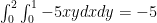 which is far more believable.
 and the planes
  ; the plane
  is outside of this cylinder. (


 find
find  That is fairly straight forward, no? But there is a bit more here than meets the eye, as I quickly found out. I graphed this on Desmos and:
 which leads to families of lines with either slope 1 or slope negative 1 and y intercepts multiples of
 which leads to:
 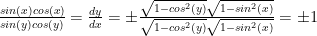 by both the original equation and the circle identity.
  so the integral is transformed into
  and so we’ve entered the realm of rational functions. Ok, ok, there is some work to do.
 be such that
  then:
then: gets transformed:
  and then
  and the integral becomes
  which is a rational function integral.
 or about 77 percent efficacy with respect to hospitalization, and
  or 93.75 percent with respect to ending up in the ICU.
 vaccines have no effect on hospitalization” vs. “effect” is
 though, of course, a series can expanded about any point in the real line (e. g.
  ) Note: unless it is needed, I’ll be suppressing the index in the summation sign.
 ..
.. only (e. g.
  ; try the ratio test) or
  for some
  and diverges for all
  (like a geometric series) (anything possible for
  ) or
) or converges (either absolute OR conditional ) So, by the divergence test, we know that the sequence of terms
  . So we can find some index
  such that
 and
and  converges absolutely for
  . The divergence follows from a simple “reversal of the inequalities (that is, if the series diverged at
  ).
). ? Of course, the function itself is continuous on the whole real line. But to find the open interval of convergence, look for the complex root of
  that is closest to zero. That would be
  so the interval is
 ) is unique:
 on the interval of convergence, then substituting
  yields
  . So subtract from both sides and get:
  . Now assuming one can “factor out an x” from both sides (and you can) we get
  , etc.
  is continuous on its open interval of absolute convergence.
 for
for  sufficiently close AND both within the open interval of absolute convergence, say
  where
where  and
and  and
and  where
where  (these are just polynomials).


 then so is
  .
. and find
  where
where  is also absolutely convergent. Now, note that
  so the series
  converges by direct comparison on
 is absolutely convergent on
  we can find
  so that
  for
for  between
  and
and 
 and then note:


 where each
  is between
  the second term is less than
  , which is arbitrary, and the first term is the first
  terms of the “expected” derivative series.
 converges and then differentiating.
  (of course,
 ![[a,b] \subset (-r, r)](https://s0.wp.com/latex.php?latex=%5Ba%2Cb%5D+%5Csubset+%28-r%2C+r%29+&bg=ffffff&fg=000000&s=0&c=20201002) )
)
 and this is less than (or equal to)
 which can be thought of as our “degree 0” expansion plus remainder term.
  (it is a clever choice for
  ; it just has to work.
 and so we have:
 .
.
 .
. for
for ![t \in [0,x]](https://s0.wp.com/latex.php?latex=t+%5Cin+%5B0%2Cx%5D+&bg=ffffff&fg=000000&s=0&c=20201002) and then
and then 
 as the error formula; it is a Mean Value Theorem for integrals calculation.
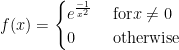
 for all
  and so a Taylor expansion at zero is just the zero function, and this is valid at 0 only.
 at
at  and substitute
  ; the uniqueness of the power series expansion allows for that.
  , the most important thing is to determine the open interval of absolute convergence; that is, the intervals on which
  converges.
  only, on some open interval
  or the whole real line. Side note: this is an interesting place to point out the influence that the calculus of complex variables has on real variable calculus! These open intervals are the most important aspect as one can prove that one can differentiate and integrate said series “term by term” on the open interval of absolute convergence; sometimes
  .
. ; here we see that for
  ,
,  and is equal to
  for
for  ; to show this do the old “shifted sum” addition:
  ,
,  then subtract:
  as most of the terms cancel with the subtraction.
  the “n’th partial sum, then the series
  converges if an only if the sequence of partial sums
  converges; yes there are
  and we get convergence if
  goes to zero, which happens only if
  .
.  has all
  (suppressing the indices).
 , then if
  is the sequence in question, there has to be some
  such that
  for any small, positive
  . Then because
  for all
 converges (standard convergence) then
  as a sequence. This is pretty clear if the
  are non-negative; the idea is that the sequence of partial sums
  becomes arbitrarily small. Of course, this is true even if the terms are not all positive.
 and
and  converges, then so does
  . If
. If  converges. Now, of course, absolute convergence implies convergence:
 and if
  converges by direct comparison. Now note
  is the difference of two convergent series:
  and therefore converges.
  is a non-negative, non-decreasing function on some
  (that is,
  ) Then
  converges if and only if
  converges as an improper integral.
 is just a right endpoint Riemann sum for
  is the right endpoint estimate for
 certainly has
  diverging.
![f(x) = \begin{cases} 2^n , & \text{ if } x \in [n, n+2^{-2n}] \\0, & \text{ otherwise} \end{cases}](https://s0.wp.com/latex.php?latex=f%28x%29+%3D+%5Cbegin%7Bcases%7D++2%5En+%2C+%26+%5Ctext%7B+if+%7D++x+%5Cin+%5Bn%2C+n%2B2%5E%7B-2n%7D%5D+%5C%5C0%2C+%26+%5Ctext%7B+otherwise%7D+%5Cend%7Bcases%7D+&bg=ffffff&fg=000000&s=0&c=20201002) gives an unbounded function with unbounded sum
gives an unbounded function with unbounded sum  but the integral converges to the sum
  . The “boxes” get taller and skinnier.
 converges if
  and diverges otherwise. Proof: Integral test.
 and
and 
 then so does
  then so does
  then
then  such that
  This means
  and we get convergence by direct comparison. See how useful that test is?
 to exist; for the convergence case it is only necessary that there be some
  ; if one is familiar with the
 clearly converges, but nailing down the proof with direct comparison can be hard. But a limit comparison with
  is pretty easy.
 (if the limit exists..if it doesn’t..stay tuned).
 the series converges. If
  the series diverges. If
  the test is inconclusive.
  such that for all
  we have
  then the series converges (we can use the
 to obtain
 See where this is going: each ratio is less than
  so we have:
 which is a convergent geometric series.
  we have
  then the series converges (exercise: find the “divergence version”).
  so the original series converges by direction comparison.
 and therefore converges by direct comparison. And the limsup version of the root test works as well.
  which is unbounded..but
  .
.  converges but does NOT converge absolutely (p-test). On one hand, such series are a LOT of fun..but the convergence is very slow and unstable and so might say that these series are not as important as the series that converges absolutely. But there is a lot of interesting mathematics to be had here.
 and for all
  .
. converges if and only if
  (as the magnitudes get steadily smaller) and below by
  (same reason. Note also that
  so the sequence of partial sums of even index are an increasing bounded sequence and therefore converges to some limit, say,
  . But
. But  and so by a routine “epsilon-N” argument the odd partial sums converge to
  as well.
  . Note: this could be 0 terms. Now use the negative terms to go of the left of
  Then move to the right, past
  . Then go back again to get
  to the left of
  and the
  bracket
  converges.
  where
where  is a
is a  matrix.
  where the powers make sense as
  is square and we merely add the corresponding matrix entries.
  can get only so large.
 (just sum up the absolute value of the elements (the Taxi cab norm or
  and
and  and together this implies the following:
 where
where  is the i-j’th element of
![| [ e^A ]_{i,j} | \leq \sum^{\infty}_{k=0} {|A^k |\over k!} \leq \sum^{\infty}_{k=0} {|A|^k \over k!} =e^{|A|}](https://s0.wp.com/latex.php?latex=%7C+%5B+e%5EA+%5D_%7Bi%2Cj%7D+%7C+%5Cleq+%5Csum%5E%7B%5Cinfty%7D_%7Bk%3D0%7D+%7B%7CA%5Ek+%7C%5Cover+k%21%7D+%5Cleq++%5Csum%5E%7B%5Cinfty%7D_%7Bk%3D0%7D+%7B%7CA%7C%5Ek+%5Cover+k%21%7D+%3De%5E%7B%7CA%7C%7D+&bg=ffffff&fg=000000&s=0&c=20201002) . Therefore every series that determines an entry of the matrix
. Therefore every series that determines an entry of the matrix 