Legendre Polynomials: elementary linear algebra proof of orthogonality

April 1, 2014

Legendre Polynomials: elementary linear algebra proof of orthogonality

Filed under: advanced mathematics, applied mathematics, calculus, integrals, linear albegra, numerical methods — Tags: Hermitian operators, Legendre polynomials, orthogonal polynomials — collegemathteaching @ 7:26 pm

In our numerical analysis class, we are coming up on Gaussian Quadrature (a way of finding a numerical estimate for integrals). Here is the idea: given an interval $[a,b]$ and a positive integer $n$ we’d like to select numbers $x_i \in [a,b], i \in \{1,2,3,...n\}$ and weights $c_i$ so that $\int^b_a f(x) dx$ is estimated by $\sum^n_{i=1} c_i f(x_i)$ and that this estimate is exact for polynomials of degree $n$ or less.

You’ve seen this in calculus classes: for example, Simpson’s rule uses $x_1 =a, x_2 = \frac{a+b}{2}, x_3 = b$ and uses $c_1 = \frac{b-a}{6}, c_2 =\frac{2(b-a)}{3}, c_3 =\frac{b-a}{6}$ and is exact for polynomials of degree 3 or less.

So, Gaussian quadrature is a way of finding such a formula that is exact for polynomials of degree less than or equal to a given fixed degree.

I might discuss this process in detail in a later post, but the purpose of this post is to discuss a tool used in developing Gaussian quadrature formulas: the Legendre polynomials.

First of all: what are these things? You can find a couple of good references here and here; note that one can often “normalize” these polynomials by multiplying by various constants.

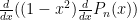
One way these come up: they are polynomial solutions to the following differential equation: $\frac{d}{dx}((1-x^2)\frac{d}{dx} P_n(x)) + n(n+1)P_n(x) = 0$ . To see that these solutions are indeed polynomials (for integer values of $n$ ). To see this: try the power series method expanded about $x = 0$ ; the singular points (regular singular points) occur at $x = \pm 1$ .

Though the Legendre differential equation is very interesting, it isn’t the reason we are interested in these polynomials. What interests us is that these polynomials have the following properties:

1. If one uses the inner product $f \cdot g = \int^1_{-1} f(x) g(x) dx$ for the vector space of all polynomials (real coefficients) of finite degree, these polynomials are mutually orthogonal; that is, if $n \ne m, P_m(x) \cdot P_n (x) = \int^1_{-1} P_n(x)P_m(x) dx = 0$ .

2. $deg(P_n(x)) = n$ .

Properties 1 and 2 imply that for all integers $n$ , $\{P_0(x), P_1(x), P_2(x), ....P_n(x) \}$ form an orthogonal basis for the vector subspace of all polynomials of degree n or less. If follows immediately that if $Q(x)$ is any polynomial of degree $k < m$ , then $Q(x) \cdot P_m(x) = 0$ ( $Q(x)$ is a linear combination of $P_j(x)$ where each $j < m$ )

Now these properties can be proved from the very definitions of the Legendre polynomials (see the two references; for example one can note that $P_n$ is an eigenfunction for the Hermitian operator $\frac{d}{dx}((1-x^2)\frac{d}{dx} P_n(x))$ with associated eigenvalue $n(n+1)$ and such eigenfunctions are orthogonal.

This little result is fairly easy to see: call the Hermitian operator $A$ and let $m \ne n, A(P_m) =\lambda_m P_m, A(P_n) =\lambda_n = A(P_n)$ and $\lambda_n \ne \lambda_m$ .

Then consider: $(A(P_m) \cdot P_n) = (\lambda_m P_m \cdot P_n) = \lambda_m (P_m \cdot P_n )$ . But because $A$ is Hermitian, $(A(P_m) \cdot P_n) = (P_m \cdot A(P_n)) = (P_m \cdot \lambda_n P_n) = \lambda_n (P_m \cdot P_n)$ . Therefore, $\lambda_m (P_m \cdot P_n ) = \lambda_n(P_m \cdot P_n)$ which means that $P_m \cdot P_n = 0$ .

Of course, one still has to show that this operator is Hermitian and this is what the second reference does (in effect).

The proof that the operator is Hermitian isn’t hard: assume that $f, g$ both meet an appropriate condition (say, twice differentiable on some interval containing $[-1,1]$ ).
Then use integration by parts with $dv =\frac{d}{dx} ((1-x^2) \frac{d}{dx}f(x)), u =g(x)$ : $\int^1_{-1} \frac{d}{dx} ((1-x^2) \frac{d}{dx}f(x))g(x) = ((1-x^2) \frac{d}{dx}f(x))g(x)|^1_{-1}-\int^1_{-1}(1-x^2)\frac{d}{dx} f(x) \frac{d}{dx}g(x) dx$ . But $((1-x^2) \frac{d}{dx}f(x))g(x)|^1_{-1} =0$ and the result follows by symmetry.

But not every student in my class has had the appropriate applied mathematics background (say, a course in partial differential equations).

So, we will take a more basic, elementary linear algebra approach to these. For our purposed, we’d like to normalize these polynomials to be monic (have leading coefficient 1).

Our approach

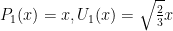
Use the Gram–Schmidt process from linear algebra on the basis: $1, x, x^2, x^3, x^4.....$

Start with $P_0 = 1$ and let $U_0 = \frac{1}{\sqrt{2}}$ ; here the $U_i$ are the polynomials normalized to unit length (that is, $\int^{1}_{-1} (U_k(x))^2 dx = 1$ . That is, $U_i(x) = \sqrt{\frac{1}{\int^1_{-1}(P_i(x))^2 dx}} P_i(x)$

Next let $P_1(x) =x, U_1(x) = \sqrt{\frac{2}{3}} x$

Let $P_2(x) = x^2 - \sqrt{\frac{2}{3}} x \int^{1}_{-1} (\sqrt{\frac{2}{3}} x)x^2 -\frac{1}{\sqrt{2}}\int^{1}_{-1} \frac{1}{\sqrt{2}}x^2 = x^2 -\frac{1}{3}$ Note that this is not too bad since many of the integrals are just integrals of an odd function over $[-1,1]$ which become zero.

So the general definition:

$P_{n+1}(x) = x^{n+1} - U_n \int^1_{-1}x^{n+1} U_n(x) dx - U_{n-1}\int^1_{-1} U_{n-1} x^{n+1}dx .... - \frac{1}{\sqrt{2}}\int^1_{-1} \frac{1}{\sqrt{2}}x^{n+1} dx$

What about the roots?
Here we can establish that each $P_m(x)$ has $m$ distinct, real roots in $(-1,1)$ . Suppose $P_m(x)$ has only $k < m$ distinct roots of odd multiplicity in $(-1,1)$ , say $x_1, x_2, ...x_k$ . Let $W(x) = (x-x_1)(x-x_2)...(x-x_k)$ ; note that $W$ has degree $k < m$ . Note that $P_m(x)W(x)$ now has all roots of even multiplicity; hence the polynomial $P_m(x)W(x)$ cannot change sign on $[-1,1]$ as all roots have even multiplicity. But $\int^{1}_{-1} P_m(x)W(x) dx = 0$ because $W$ has degree strictly less than $m$ . That is impossible. So $P_m(x)$ has at least $m$ distinct roots of odd multiplicity, but since $P_m(x)$ has degree $m$ , they are all simple roots.

Comments (3)

3 Comments »

[…] haven’t written much except to record my workouts…at least here. I did write this post yesterday (on my math […]

Pingback by Blogging: light « blueollie — April 2, 2014 @ 11:17 am

Reply
[…] a previous post, I discussed the Legendre polynomials. We now know that if is the n’th Legendre polynomial […]

Pingback by Gaussian Quadrature and Legendre polynomials | College Math Teaching — April 4, 2014 @ 2:08 am

Reply
[…] Base from: College Math Teaching […]

Pingback by Legendre Polynomials: elementary linear algebra proof of orthogonality | Ragnarok Connection — July 10, 2014 @ 1:35 am

Reply

RSS feed for comments on this post. TrackBack URI

College Math Teaching

April 1, 2014